Thomas Kloecker Betreuer: Tim Priesnitz

Spracherkennungs-und Anfrage-Aequivalenz von MSO, monadischem Datalog, und Automaten.
Thomas Kloecker Betreuer: Tim Priesnitz Seminar Logische Aspekte von XML, Gerd Smolka, PS Lab, Uni Saarland, SS 2003

Uebersicht • 'algebraisch' vs. • deterministisch?
0. Datalog vs. SQL; monadischer Datalog 1. Automaten  monadischer Datalog 2. Monadischer Datalog  MSO 3. MSO  Automaten Universum Automatentypen A. Strings B. Ranked Trees C. Unranked Trees • 'algebraisch' vs. bottom-up vs. top-down. • deterministisch?

Uebersicht • Sprach-erkennung • Query-Berechnung
0. Datalog vs. SQL; monadischer Datalog 1. Automaten  monadischer Datalog 2. Monadischer Datalog  MSO 3. MSO  Automaten Universum Automatentypen Aufgabe A. Strings B. Ranked C. Unranked 'normal' vs. two -way deterministisch • Sprach-erkennung • Query-Berechnung

Automaten, monadischer Datalog & MSO

Presburger Arithmetik
Datalog - Beispiel Presburger Arithmetik q0 q1 1  ... q2 q0 q0 q0 q1 q0 q2 Endlicher Automat für Addition

Datalog - Beispiel nocar(0). in_101(0).
nocar(NextPos) :- s(Pos, NextPos), nocar(Pos), in_000(Pos). % = 0+0 nocar(NextPos) :- s(Pos, NextPos), nocar(Pos), in_011(Pos). % = 1+0 nocar(NextPos) :- s(Pos, NextPos), nocar(Pos), in_101(Pos). % = 1+0 nocar(NextPos) :- s(Pos, NextPos), carry(Pos), in_001(Pos). % = 1+0 % c+x+y = z+c' carry(NextPos) :- s(Pos, NextPos), carry(Pos), in_010(Pos). % = 0+1 carry(NextPos) :- s(Pos, NextPos), carry(Pos), in_100(Pos). % = 0+1 carry(NextPos) :- s(Pos, NextPos), carry(Pos), in_111(Pos). % = 1+1 carry(NextPos) :- s(Pos, NextPos), nocar(Pos), in_110(Pos). % = 0+1 endOfFile(NextPos) :- s(Pos, NextPos), in_BotBotBot(Pos). accept :- endOfFile(_). in_101(0). in_011(1). in_110(2). in_001(3). in_BotBotBot(4). s(0,1). s(1,2). s(2,3). s(3,4). s(4,5).

Datalog Beispiel Presburger Arithmetik
nocar(0). nocar(NextPos) :- s(Pos, % c+x+y = z+c' carry(NextPos) :- s(Pos, NextPos), carry(Pos), in_010(Pos). % = 0+1 carry(NextPos) :- s(Pos, NextPos), carry(Pos), in_100(Pos). % = 0+1 carry(NextPos) :- s(Pos, NextPos), carry(Pos), in_111(Pos). % = 1+1 carry(NextPos) :- s(Pos, NextPos), nocar(Pos), in_110(Pos). % = 0+1 endOfFile(NextPos) :- s(Pos, NextPos), in_BotBotBot(Pos). accept :- endOfFile(_). in_101(0). in_011(1). in_110(2). in_001(3). in_BotBotBot(4). s(0,1). s(1,2). s(2,3). s(3,4). s(4,5). 1  ...

nocar(0). nocar(NextPos) :- s(Pos, NextPos), nocar(Pos), in_000(Pos). % = 0+0 nocar(NextPos) :- s(Pos, NextPos), nocar(Pos), in_011(Pos). % = 1+0 nocar(NextPos) :- s(Pos, NextPos), nocar(Pos), in_101(Pos). % = 1+0 nocar(NextPos) :- s(Pos, NextPos), carry(Pos), in_001(Pos). % = 1+0 % c+x+y = z+c' carry(NextPos) :- s(Pos, NextPos), carry(Pos), in_010(Pos). % = 0+1 carry(NextPos) :- s(Pos, NextPos), carry(Pos), in_100(Pos). % = 0+1 carry(NextPos) :- s(Pos, NextPos), carry(Pos), in_111(Pos). % = 1+1 carry(NextPos) :- s(Pos, NextPos), nocar(Pos), in_110(Pos). % = 0+1 endOfFile(NextPos) :- s(Pos, NextPos), in_BotBotBot(Pos). accept :- endOfFile(_). in_101(0). in_011(1). in_110(2). in_001(3). in_BotBotBot(4). s(0,1). s(1,2). s(2,3). s(3,4). s(4,5).

in_101(0). in_011(1). in_110(2). in_001(3). in_BotBotBot(4). s(0,1). s(1,2). s(2,3). s(3,4). s(4,5). nocar(0). nocar(NextPos) :- s(Pos, NextPos), nocar(Pos), in_000(Pos). % = 0+0 nocar(NextPos) :- s(Pos, NextPos), nocar(Pos), in_011(Pos). % = 1+0 nocar(NextPos) :- s(Pos, NextPos), nocar(Pos), in_101(Pos). % = 1+0 nocar(NextPos) :- s(Pos, NextPos), carry(Pos), in_001(Pos). % = 1+0 % c+x+y = z+c' carry(NextPos) :- s(Pos, NextPos), carry(Pos), in_010(Pos). % = 0+1 carry(NextPos) :- s(Pos, NextPos), carry(Pos), in_100(Pos). % = 0+1 carry(NextPos) :- s(Pos, NextPos), carry(Pos), in_111(Pos). % = 1+1 carry(NextPos) :- s(Pos, NextPos), nocar(Pos), in_110(Pos). endOfFile(NextPos) :- s(Pos, NextPos), in_BotBotBot(Pos). accept :- endOfFile(_). nocar carry endOfFile

Datalog accept :- endOfFile(_).
in_101(0). in_011(1). in_110(2). in_001(3). in_BotBotBot(4). s(0,1). s(1,2). s(2,3). s(3,4). s(4,5). nocar(0). nocar(NextPos) :- s(Pos, NextPos), nocar(Pos), in_000(Pos). % = 0+0 nocar(NextPos) :- s(Pos, NextPos), nocar(Pos), in_011(Pos). % = 1+0 nocar(NextPos) :- s(Pos, NextPos), nocar(Pos), in_101(Pos). % = 1+0 nocar(NextPos) :- s(Pos, NextPos), carry(Pos), in_001(Pos). % = 1+0 % c+x+y = z+c' carry(NextPos) :- s(Pos, NextPos), carry(Pos), in_010(Pos). % = 0+1 carry(NextPos) :- s(Pos, NextPos), carry(Pos), in_100(Pos). % = 0+1 carry(NextPos) :- s(Pos, NextPos), carry(Pos), in_111(Pos). % = 1+1 carry(NextPos) :- s(Pos, NextPos), nocar(Pos), in_110(Pos). endOfFile(NextPos) :- s(Pos, NextPos), in_BotBotBot(Pos). accept :- endOfFile(_). nocar carry endOfFile

Datalog - Grundlegende Konzepte
• Extensionaler und intensionaler Programmteil • kurzer Vergleich mit SQL • formale Definition • Dialekte • basic vs. stratified • monadisch / voll • Prolog • Semantik

Datalog vs SQL SQL Datalog Typen
Schema = Menge von Namen von Relationen und Attributen Signatur = Namen und Aritaeten der extensionalen Praedikate Modellierung von gespeichert vs berechnet Tables vs Views Extensionale Datenbank (EDB) vs Intensionale Datenbank (IDB) Expressivitaet Transitiver Abschluss nicht modellierbar Turing complete.

Datalog vs SQL SQL - tables SQL - views Datalog- Signatur
Getraenke(gid, name, preis) Kunden(tid, tname, schuhgroesse) Konsum(gid, tid, menge, datum) SQL - views Kunde2(tid, kontonummer) Konsum2(name, preis, menge, datum, schuhgroesse) SELECT blahblah Datalog- Signatur (getraenk, kunde, konsum) kunde(17, hans, 46). kunde(18, maria, 40). mensch(sokrates). mensch(hans). Datalog- Regeln Alle Menschen sind sterblich. sterblich(X) :- mensch(X). Wenn Hans 2 Paar Schuhe hat, verkauft er das teurere Paar. verkauft(hans, X) :- hat(hans,X), hat(hans,Y), schuh(X), schuh(Y), X\==Y, teurerAls(X,Y).

Datalog - Interaktion / Anfragen
1 ?- sterblich(sokrates). yes.

1 ?- sterblich(sokrates). yes. 2 ?- sterblich(X). X = sokrates;

1 ?- sterblich(sokrates). yes. 2 ?- sterblich(X). X = sokrates; X = hans;

1 ?- sterblich(sokrates). yes. 2 ?- sterblich(X). X = sokrates; X = hans; no.

1 ?- sterblich(sokrates). yes. 2 ?- sterblich(X). X = sokrates; X = hans; no. 3 ?- sterblich(_).

Datalog - formale Definition
• Signatur = dasselbe wie ranked Alphabet (Datalog - Sprechweise) • Sei eine Signatur  gegeben. Ein einfaches Datalog Programm (ueber ) mit intensionalen Praedikaten PI ist eine Menge von Regeln der Form H :- B1, …, Bn. (wobei die linke Seite H Head, und die rechte Seite B1, …, Bn Body, genannt werden), wenn gilt: 1) Alle Heads sind in Atome Ru1,.., un mit R in PI . 2) Alle Bj , 1 <= j <= n, sind entweder Atome Ru1,.., un mit R in PI , oder Literale (¬)Ru1,.., un mit R in  , 3)   PI = 

• Die Elemente von  heissen auch extensionale Praedikate oder Input Praedikate. Das einfache Datalog Program selbst heisst auch intensionale Datenbank, oder IDB. • Eine Regel wie die obige, jedoch mit leerem Body, und als Head ein Atom Ru1,.., un mit R aus , heisst auch ein Fakt. Mengen von Fakten heissen auch extensionale Datenbank, oder EDB. • Die Semantik des Programms (d.h. der IDB) ist eine Abbildung EDB  Zuweisung von Wahrheitswerten an die intensionalen Praedikate. • Ein stratifiziertes Datalog Programm ist eine geordnete Folge von einfachen Datalog Programmen, Strata genannt. Jedes Stratum wird als EDB (d.h. Input) des naechsthoeheren Stratums interpretiert.

• Ein Datalog Programm heisst monadisch, wenn alle intensionalen Praedikate Aritaet 1 haben. • Die Signatur fuer monadischen Datalog auf ranked trees gemaess Gottlob/Koch ist: ( root, leaf, (childk)k <= maxAritaet, (labela) a  , ) • Die Signatur fuer monadischen Datalog auf unranked trees gemaess ( root, leaf, (labela) a   ) firstChild, lastChild, nextSibling)

Datalog - Semantik EDB IDB Interactive Toplevel mensch(sokrates).
sterblich(X) :- mensch(X). Interactive Toplevel 1 ?- sterblich(sokrates). yes. 2 ?- sterblich(thomas). no.

Datalog - Semantik shaves(barber, X) :- ¬shaves(X, X).
1 ? - shaves(cartman, cartman). no. 2 ? - shaves(barber, cartman). yes. 3 ? - shaves(barber, barber). ERROR: out of local stack

Datalog - Semantik Kleinster Fixpunkt (Perfect Model)
• Erste Wahl: Kleinster Fixpunkt (Perfect Model) • Existiert fuer einfaches Datalog • Im stratified Fall Semantik hierarchisch / schrittweise; kleinster Fixpunkt existiert nicht.

Datalog - stratified %% search.pl -- Section 2.16 of Prolog Tutorial
solve(P) : start(Start), search(Start,[Start],Q), reverse(Q,P). search(S,P,P) :- goal(S) /* done */ search(S,Visited,P) :- next_state(S,Nxt), /* generate next state */ safe_state(Nxt), /* check safety */ no_loop(Nxt,Visited), /* check for loop */ search(Nxt,[Nxt|Visited],P). /* continue searching... */ no_loop(Nxt,Visited) : \+member(Nxt,Visited). start([]). goal(S) :- length(S,8). next_state(S,[C|S]) :- member(C,[1,2,3,4,5,6,7,8]), \+member(C,S). safe_state([C|S]) :- length(S,L), Sum is C+L+1, Diff is C-L-1, safe_state(S,Sum,Diff). safe_state([],_,_) :- !. safe_state([F|R],Sm,Df) :- length(R,L), X is F+L+1, X \= Sm, Y is F-L-1, Y \= Df, safe_state(R,Sm,Df).

Automaten  monadischer Datalog
• ranked trees: Beispiel: d(neg(0), or(0, 1)) Signatur: ( root, leaf, (childk)k <= maxAritaet, (labela) a  , ) lblAND(root). lblNOT(root-1). lblFALSE(root-1-1). lblOR(root-2). lblTRUE(root-2-2). lblFALSE(root-2-1). root(root). child_1(root, root-1). child_2(root, root-2). child_1(root-1, root-1-1). child_1(root-2, root-2-1). child_2(root-2, root-2-2).

accept :- truth(root). false(Pos) :- lblFALSE(Pos). truth(Pos) :- lblTRUE(Pos). false(Pos) :- lblAND(Pos), child_1(Pos, ChildPos), false(ChildPos). false(Pos) :- lblAND(Pos), child_2(Pos, ChildPos), false(ChildPos). truth(Pos) :- lblAND(Pos), child_1(Pos, ChildPos_1), child_2(Pos, ChildPos_2), truth(ChildPos_1), truth(ChildPos_2). truth(Pos) :- lblOR(Pos), child_1(Pos, ChildPos), truth(ChildPos). truth(Pos) :- lblOR(Pos), child_2(Pos, ChildPos), truth(ChildPos). false(Pos) :- lblOR(Pos), child_1(Pos, ChildPos_1), child_2(Pos, ChildPos_2), false(Pos-1), false(Pos-2). truth(Pos) :- lblNOT(Pos), child_1(Pos, ChildPos), false(ChildPos). false(Pos) :- lblNOT(Pos), child_1(Pos, ChildPos), truth(ChildPos).

Definition: Gegeben ein monadisches Datalog-Programm P ueber ranked trees mit ausgezeichnetem Praedikat accept, und mit LEERER EDB. Fuer einen Sigma-gelabelten Baum T definiere edb(T) := Uebersetzung von T in TauRanked(Sigma) Schreibweise, P(T) := das Datalog Programm mit IDB P und EDB edb(T), und M(P(T)) := das eindeutig bestimmte minimale Modell von P(T) dann ist die von P erkannte Sprache L(P)  (N* -> Sigma)r-Baum definiert durch T in L(P) <==> M(P(T)) |= accept. ( In der Praxis: T in L(P) <==> Prolog (oder sonstige Implementierung) antwortet "yes" auf die Frage "accept." ) Gegeben ein deterministischer Baumautomat A ueber Sigma, mit Zustandsmenge Q, und Uebergangsfunktionen Delta(Sigma) in Q^n -> Q fuer sigma in Sigma und ar(sigma) = n. Satz (Gottlob) es ex ein monadisches Datalog-Programm P, derart dass L(P) = L(A)

Beweis / Konstruktion: * Fuer jedes q in Q intensionales Praedikat, ebenfalls q genannt. * Fuer sigma in Sigma, ar(sigma) = n, q-bar = (q1,...,qn) in Q^n, sei die Regel R(sigma, Q-bar) wie folgt definiert ( wobei delta(sigma)(q-bar) = q ) q(Pos) :- label_sigma(Pos), child(Pos, ChildPos1), q1(ChildPos1), * Fuer Endzustaende q definiere die Regel R_fin(q) durch accept :- q(root). Fuer jede Regel deltaaccept :- truth(root).

Gegeben ein deterministischer Baumautomat A ueber Sigma, mit Zustandsmenge Q, und Uebergangsfunktionen Delta(Sigma) in Q^n -> Q fuer sigma in Sigma und ar(sigma) = n. Satz (Gottlob) es ex ein monadisches Datalog-Programm P, derart dass L(P) = L(A) Beweis / Konstruktion: * Fuer jedes q in Q intensionales Praedikat, ebenfalls q genannt. * Fuer sigma in Sigma, ar(sigma) = n, q-bar = (q1,...,qn) in Q^n, sei die Regel R(sigma, Q-bar) wie folgt definiert ( wobei delta(sigma)(q-bar) = q ) q(Pos) :- label_sigma(Pos), q1(Pos-1),...,qn(Pos-n) ( verkuertzt Schreibweise ) q(Pos) :- label_sigma(Pos), child(Pos, ChildPos1), q1(ChildPos1), ( geschwaetzige Schreibweise ) * Fuer Endzustaende q definiere die Regel R_fin(q) durch accept :- q(root). Fuer jede Regel deltaaccept :- truth(root). false(Pos) :- lblFALSE(Pos). truth(Pos) :- lblTRUE(Pos). false(Pos) :- lblAND(Pos), child_1(Pos, ChildPos), false(ChildPos). false(Pos) :- lblAND(Pos), child_2(Pos, ChildPos), false(ChildPos). truth(Pos) :- lblAND(Pos), child_1(Pos, ChildPos_1), child_2(Pos, ChildPos_2), truth(ChildPos_1), truth(ChildPos_2). truth(Pos) :- lblOR(Pos), child_1(Pos, ChildPos), truth(ChildPos). truth(Pos) :- lblOR(Pos), child_2(Pos, ChildPos), truth(ChildPos). false(Pos) :- lblOR(Pos), child_1(Pos, ChildPos_1), child_2(Pos, ChildPos_2), false(Pos-1), false(Pos-2). truth(Pos) :- lblNOT(Pos), child_1(Pos, ChildPos), false(ChildPos). false(Pos) :- lblNOT(Pos), child_1(Pos, ChildPos), truth(ChildPos).

Contribution • theorem:
satisfiability of structural subtyping constraints for recursive types is DEXPTIME complete. • new relationship to modal logics • extension of Wand & Tiuryn´s appoach

Spracherkennung vs. Anfragen
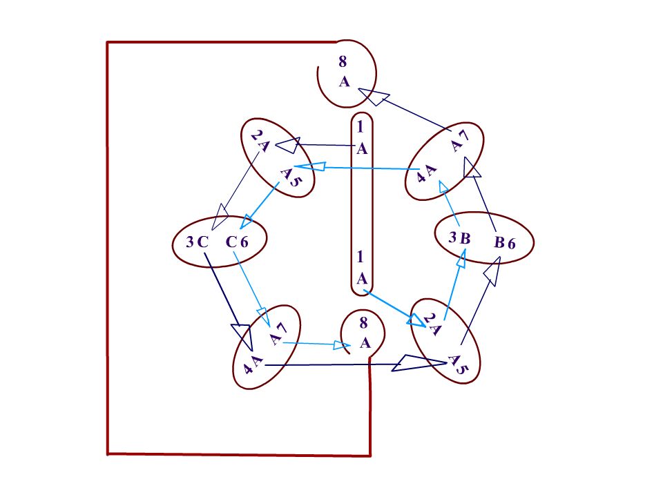
Sprache  Baeume   Anfrage  Baeume  (  ( Knoten   ) ) Korrespondenz Automaten <--> MSO hochheben auf • Anfragen • unranked case conclusion

Position 1 2 3 4 5 6 7 8 U A B C V

forth(4) back(7)

Related Work • subtype constraints for programming languages
[Mitchell 91] • logical problems: satisfiability, [Fuh, Mishra 90, Amadio, Cardelli 93, Eifrig, Smith, Trifonow ] entailment, and [Pottier 98, Rehof, Henglein 97, Niehren, Priesnitz] first-order validity [Aiken, Zu, Niehren, Priesnitz, Treinen, Kuncak] • satisfiability checking for type reconstruction

forth(4) back(7)

Contribution • theorem:
satisfiability of structural subtyping constraints for recursive types is DEXPTIME complete. • new relationship to modal logics • extension of Wand & Tiuryn´s appoach

Types • basic types int, real • function types • pair types
• polymorphic types x. xx [Milner]  pair int  int int

Types are Trees signature of function symbols a,b,f f f a f a a f a f
. a b . . a constants only finite trees (ground terms) infinite trees f ( a , f(a,b) )

Subtyping • subtypes (substitution) int ≤ real [Mitchell 91]
• ordering is lifted to ground terms Example: a ≤ b f(a,a) ≤ f(a,b) t1 ≤ s t2 ≤ s2 f(t1, t2) ≤ f(s1, s2)

Structural versus Non-Structural
f f b f a b f f  f a f ≤ ≤ f a b     ≤ τ ≤ τ for every tree τ

Constraint Languages • terms t over basic types,
smallest/greatest types ?, function (pair) types, and type variables • subtype constraints are conjunctions of inequations t1 ≤ t2

Open Questions • Is entailment of non-structural subtyping decidable?
- structural case solved [Rehof, Henglein 97,98] - many approaches [Niehren, Priesnitz, Aiken, Zu, Treinen] • satisfiability of subtyping with constant ordering - complexity for structural subtyping with recursive types [Wand, Tiuryn: between PSPACE and DEXPTIME] - decidability for non-structural subtyping

Structural Subtyping with Constants
• constant ordering is lattice: O(n ) [Kozen, Palsberg, Schwartzbach 94, Palsberg, Wand, O’Keefe 97] • arbitrary ordering 3 lower bound upper bound constants only NP-hard in NP finite trees PSPACE-hard in PSPACE infinite trees DEXPTIME-hard in DEXPTIME Pratt, Tiuryn 93, easy Tiuryn, Wand Frey 2002 new! Tiuryn, Wand 93

Example: NP-hardness signature with 4 constants
a b c d signature with 4 constants c < a, c < b, d < a, d < b a x’ b x y c y’ d consider constraint c ≤ x ≤ a  d ≤ y ≤ b  y’ ≤ x ≤ x’  y’ ≤ y ≤ x’ a x=x’=b a=x=x’ b which has exactly 2 solutions: c=y’=y d c y’=y=d

Negation Gate a z1 z2 b x z3 z4 y c z5 z6 d true z1 z2 b b z7 true
has exactly 2 solutions: a=z3=z2, b=z4=z1, c=x=z5, d=y=z6 a=x=z1, b=y=z2, c=z4=z6, d=z3=z5 true z z b b z7 true negation gate: x = z x z z y y z false z z6 d d z8 false plug it together

Negation Gate for Vectors
f true f false f false f false f false f false f true f true f true . . . . . . . . .  * true false false false false false true true true . . . . . . . . .  * constants are unary

Negation Gate: Implementation
• new variables: a∞ a∞ = a ( a∞ ) • x is boolsche: false∞ ≤ x ≤ true∞ • same idea to implement  only negate at position π  negate all positions at π1* a a a . π π *

Example: 1-Bit-Counter
true a given signature with 4 unary symbols false b define counter by true false true∞ ≤ x ≤ false∞  true∞ ≤ y ≤ false∞  x= y  x=true(y) false true true false false true x y

Regular Tree Constraints: Models
Complete Infinite Tree. x y x y x y 1 2 1 x y 2 x y 1 2  x  y x y  x  y  x  y alternative: v  {true,false} for π in (1∪2)* π

Regular Tree Constraints
given signature with constant ordering, alphabet A of letters i, regular expressions r over A, regular tree constraints are conjunctions of 4 types • ( x ≤ y ) • ( x ≤ c ) • ( c ≤ x ) π πi π in r πi π π in r π π in r π π in r

Tiuryn & Wand’s Approach
Satisfiability of structural subtype constraints over infinite trees is O(n)-reducible to regular tree constraints. Tiuryn, Wand 93

Propositional Dynamic Logic (PDL)
• Pratt’s dynamic logic • logic for program verification • propositional fragment by Fischer, Ladner

PDL Models models are rooted directed labeled graphs x y x y x y 2
1 2 x  y x y x y 1,2 2 2  x  y models are rooted directed labeled graphs

PDL Language • alphabet A = { 1,2,...n }
• regular expressions r over A • PDL Syntax: φ ::= P  φ  φ  φ’  [r] φ • modal operator [r] φ for all r-sucessors holds φ 1 P Q 2 P Q [1∪2] (PQ)

Example: 1-Bit-Counter
+ [1*] (P ∨ [1] P)  P has one solution in the class of unary infinite deterministic trees P 1 P 1 P 1 P 1

Tree PDL models are restricted to be functional
1 2 1 2 1 2 theorem: satisfiability of Tree PDL is DEXPTIME-complete proof: reduction to deterministic PDL: models are restricted to be functional 1,2 2 2 forbidden Satisfiability of Deterministic PDL is DEXPTIME-complete. Ben-Ari, Halpern, Pnueli 82 & Parikh 78

Regular Tree Constraints  Tree PDL
theorem: regular tree constraints are a fragment of tree DPL example signature x ≤ y  Px  Py • ( x ≤ y )  [r] (Px  [i]Py) • ( x ≤ false )  [r] (Px  false) true false ε ε π πi π in r π π in r

Core Tree PDL Core Tree PDL is defined by a restricted syntax:
φ ::= [r1]ψ1  …  [rn]ψn where r is ε or (1∪2)* ψ ::= P  ψ  ψ  ψ  [r] ψ where r is 1 or 2

Satisfiability of Core Tree PDL
theorem: satisfiability of Core Tree PDL is DEXPTIME-complete possibilities for the hardness-proof: encode • Halting-Problem of alternating linear-space bounded Turing machine. • Exists a winning strategy in a two person tiling game? Maarten de Rijke: PDL • Emptiness of the intersection of some tree automta. Helmut Seidl: haskell overloading

Sat. of Core Tree PDL is DEXPTIME-hard
regard n tree automata (Q, Σ, δ, q ) with Σ = { f, a, b } init except one nonempty infinite tree [(1∪2)*] ( Pf ∨ Pa ∨ Pb ∨ P#) [(1∪2)*] (Pa ∨ Pb ∨ P#)  [1∪2] P# [ε]  P# Pf Pa Pb P# P# P# P# a b f + except one nonempty finite tree mark with counter all exponential deep nodes [(1∪2)*] Pdeep  P# Pf Pa Pb Pdeep PdeepPdeep Pdeep

Sat. of Core Tree PDL is DEXPTIME-hard
every tree automata accepts a tree [ε] Pq Pqinit Pq2 Pq1 Pq1 Pq1 Pq1 init [(1∪2)*] (Pf ∧ [1] Pq ∧ [2] Pq’ )  Pq’’ if f(q,q’) q’’ in δ [(1∪2)*] Pa  Pq if a q in δ init

Core Tree PDL  Subtype Constraints
main theorem: sat. of core tree PDL is O(n)-reducible to sat. of structural subtype constraints over infinite trees. reduce example: [(1∪2)*] (P  [i]P’) [*] P2= (P  P1= ( [i] P’ ) ) [*] P2 = (P  P1 = ( [i] P’ ) ) false∞ ≤ { P2, P, P1, P’ } ≤ true∞  P1=true( P‘)  P2 = P  P1  P2=true ∞ * * * * *i *

Conclusion • modal logic approach to subtyping constraints
• non-structural case still open • can we extend our approach? • what about entailment?

thank you I work together with Joachim Niehren on the question
whether or not the so called Non-Structural Subtype Entailment problem is decidable. There has been started a lot of attacks but the problem is still open.

Result Pratt, Tiuryn 96 Satisfiability of Structural Subtype Constraints is NP-complete in the Model of single Leafs (Signature contains only Constants)

Thomas Kloecker Betreuer: Tim Priesnitz

Ähnliche Präsentationen

Präsentation zum Thema: "Thomas Kloecker Betreuer: Tim Priesnitz"— Präsentation transkript:

Ähnliche Präsentationen

Über Projekt

Feedback

Anmelden

Anmeldung über soziales Netzwerk:

Thomas Kloecker Betreuer: Tim Priesnitz

Ähnliche Präsentationen

Präsentation zum Thema: "Thomas Kloecker Betreuer: Tim Priesnitz"— Präsentation transkript:

Ähnliche Präsentationen

Über Projekt

Feedback