The use of copulas for the description of the spatial variability of environmental variables András Bárdossy Universität Stuttgart.

Präsentation zum Thema: "The use of copulas for the description of the spatial variability of environmental variables András Bárdossy Universität Stuttgart."—  Präsentation transkript:

1 The use of copulas for the description of the spatial variability of environmental variables
András Bárdossy Universität Stuttgart

2

3

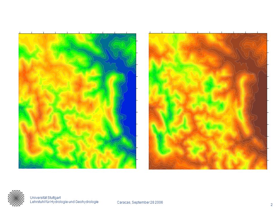
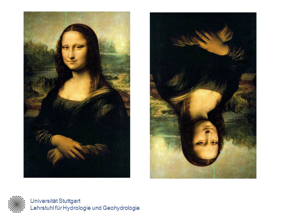
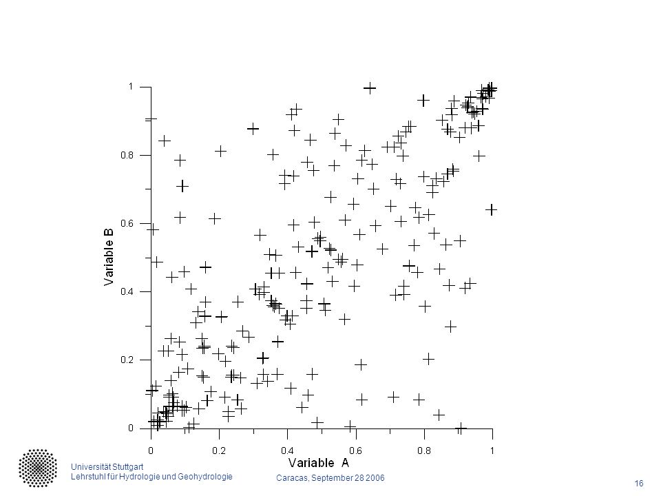
4 Spatial patterns are not necessarily symmetrical

5 Paul Klee: Copula

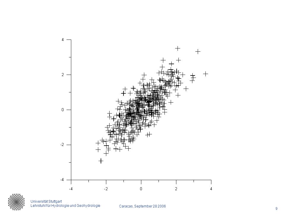
6 Dependence Goal: dependence between two variables: To recognize
To quantify Correlation (Signifikance Normal distribution) Linear Regression

7

8

9

10

11

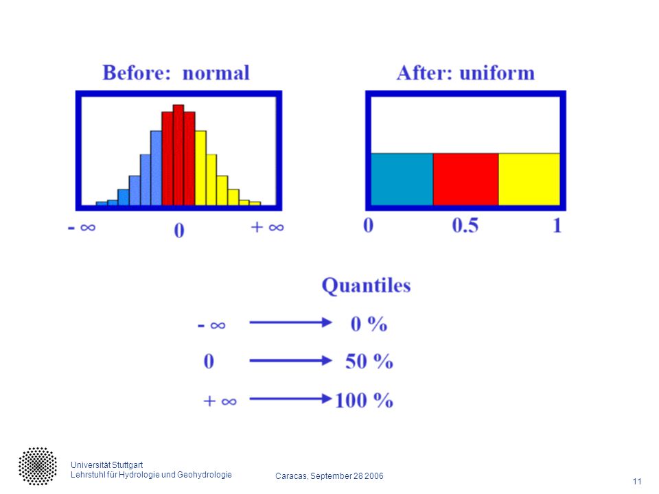
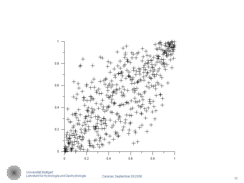
12 Dependence changes through a Transformation of the Marginal distribution
Correlations between 0.4 and 0.8 Idea: take the same marginal distribution Uniform in [0,1] Transformation using the pdf

13

14 Dependence  Marginal distributions

15 Bivariate Distributions and Copulas
Bivariate Copula = bivariate pdf with uniform marginals

16

17 Copulas are a new way of modelling the correlation structure between variables.
They dissociate the correlation structure from the marginal distributions of the individual variables.

18 Entropy = measure of Information (Shannon)
Differential entropy: Conditional Differential entropy Interesting for „extreme“ (v large)

19 Multivariate Distributions and Copulas
Sklar (1959) all F pdf can be written in this form and C is unique if F is continuous Measures of the dependence Differential Entropy Rank correlation (Spearman) Kendalls tau

20 Copula density

21 Multivariate normal copula
Copula density:

22 Normal copula

23 Can copulas be used for the description of spatial variability ?
Do we need this ?

24 Geostatistics Z(x) Random function – Realisation z(xi)
Assumption – „uniform continuity“ No differences are known a-priori Independent of the location – depends only on h (Semi)Variogramm  Covariance function

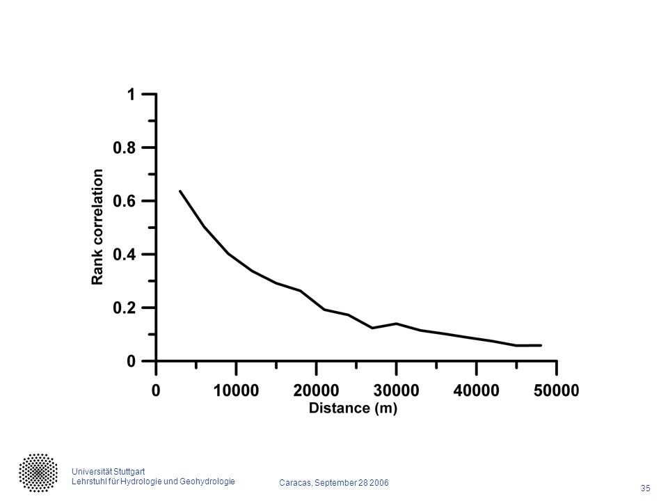
25 Experimental Variogramm EC

26 Spatial copulas Assumption:
Multivariate copula exists for any number of points The bi-variate marginal copulas corresponding to pairs separated by a vector h are translation invariant How to find such copulas ?

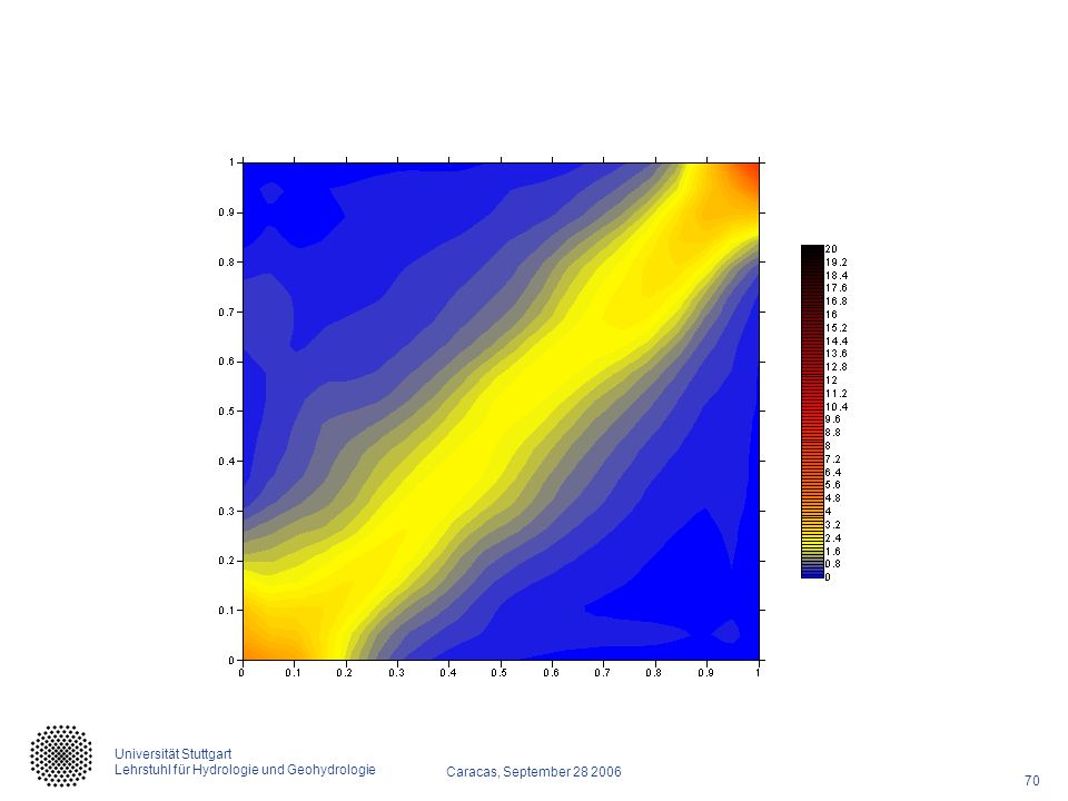
27 Empirical copulas Set of pdf pairs corresponding to points separated by the vector h Generalization of the variogram Empirical density using kernel smoothing

28

29

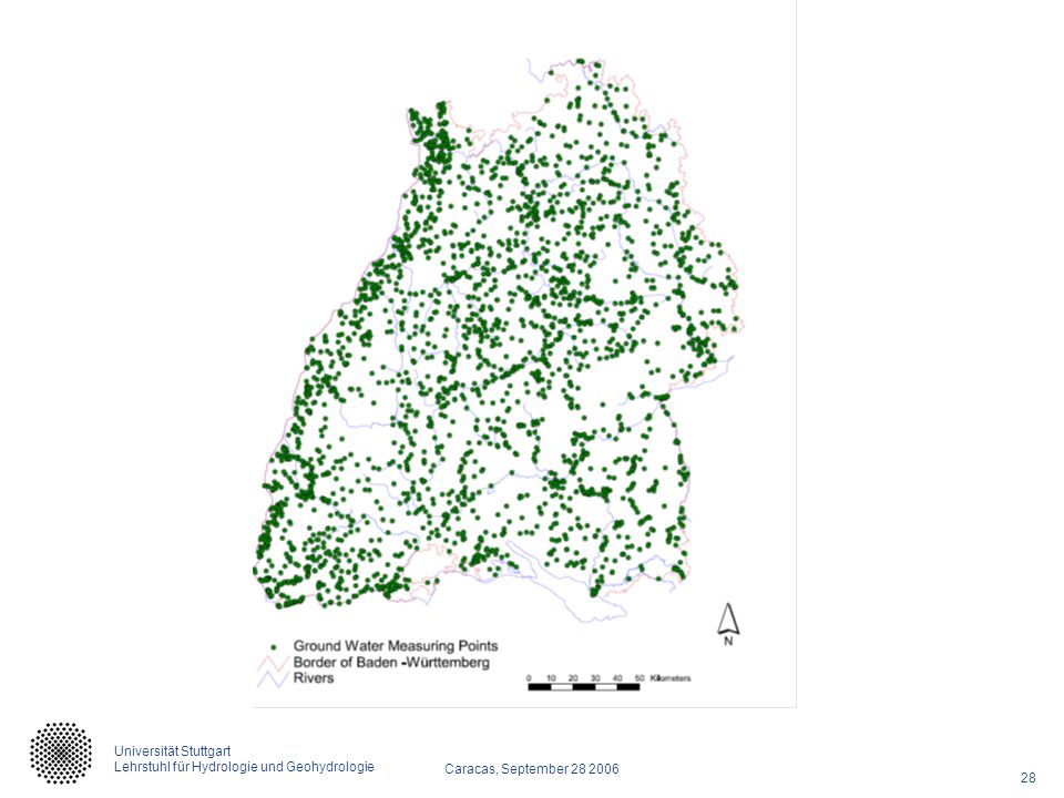
30 Nitrat und Phosphat

31 Copula Nitrate GW 5 km

32 Entropy: Nitrat m und 30000m

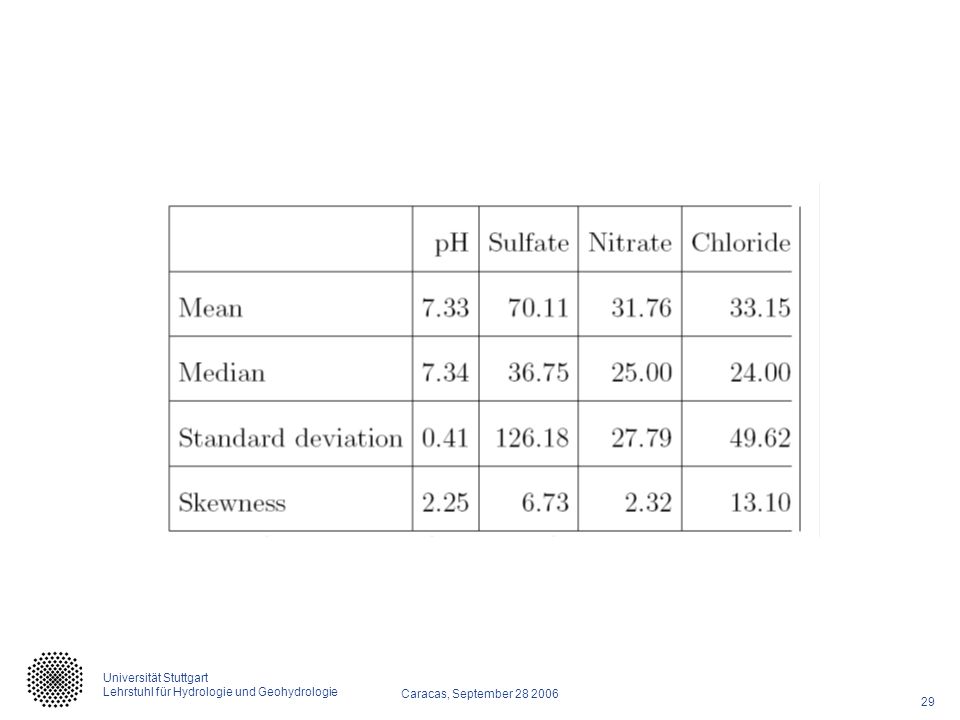
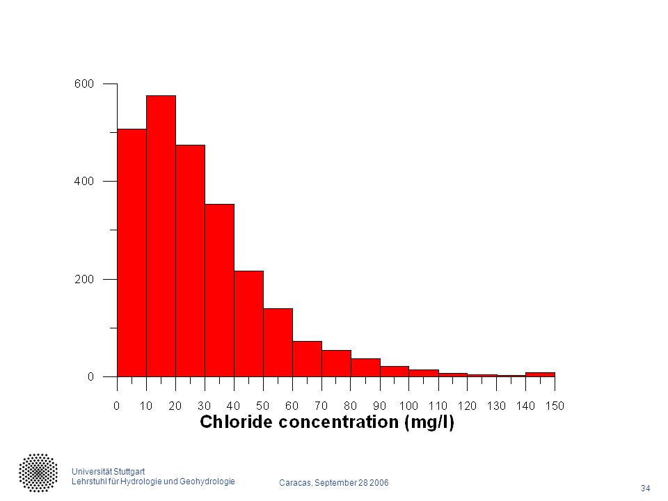
33 Cl Variogramm

34

35

36 Copula pH groundwater

37 pH Variogramm

38

39

40 n-dimensional Chi-square copula

41 Chi-Quadrat Copulas

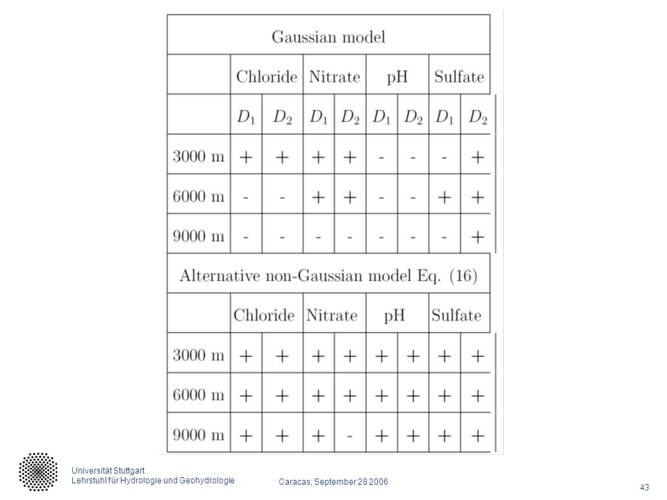
42 Testing the multivariate copulas
Analytically difficult due to the dependence of the pairs Simulation and Bootstrap to compare bi-variate marginals to theoretiacal

43

44 Summary and conclusions Copulas offer an interesting alternative Many natural variables show a non-Gaussian spatial dependence

45 Thank you ! PS: I have another 253 slides to show – maybe next time !
On behalf of the Insurance Leadership Institute, Welcome. GE Insurance Solutions’ Institute is the place for people within our industry, from around the world to come together. To learn. To network. To develop. Our focus is to help you learn practical skills and solutions; Network with each other to build and strengthen relationships; and Develop your expertise to achieve better business results. While The Institute is physically located at our Corporate Headquarters in Kansas City, Missouri in the United States. We are connected globally.

46 Indikator Variablen Indikator variablen Indikator variogram

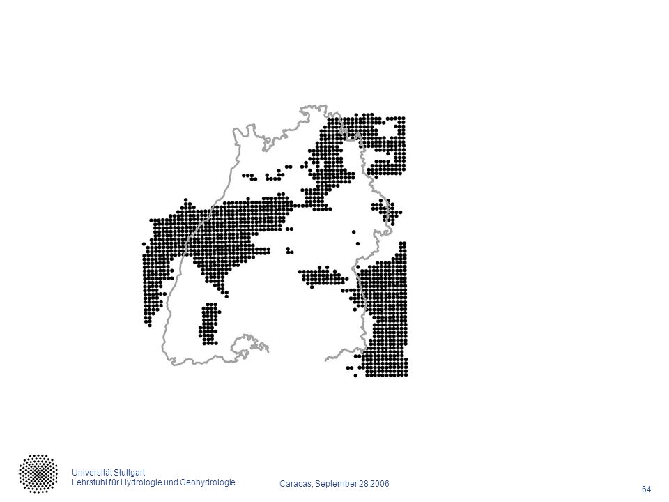
47 Spatial dependence – 5 km Event 70

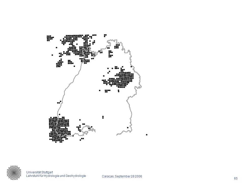
48 Spatial dependence – 5 km Event 347

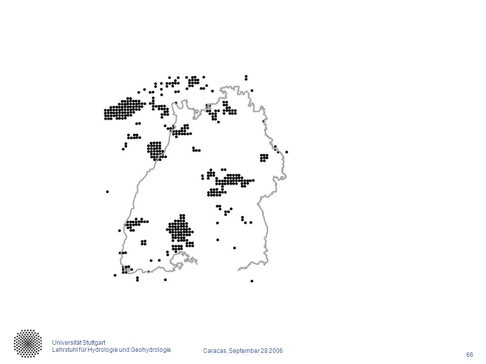
49 Spatial dependence – 5 km Event 159

50 Radarniederschlag 29. Dezember 2001 11:20-13:20

51 Copula Radarniederschlag 29. Dezember 2001 11:20-13:20

52 Gauss – Chi-square

53

54 Statistische Tests Problem: Paare sind nicht unabhängig
Deshalb klassische Tests nicht verwendbar Lösung: Bootstrap

55 Zusammenfassung Zusammenhänge können mit Copulas „einheitlich“ quantifiziert werden Viele natürliche Parameter zeigen assymetrische Zusammenhänge Diese Eigenschaft kann bei der räumlichen Betrachtung berücksichtigt werden

56

57 Simulation results

58 Räumlicher Zusammenhang – 5 km Ereignis 71

59 Räumlicher Zusammenhang – 5 km Ereignis 117

60 Räumlicher Zusammenhang – 5 km Ereignis 348

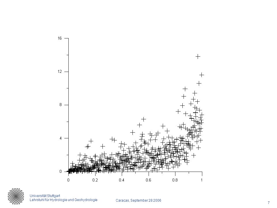
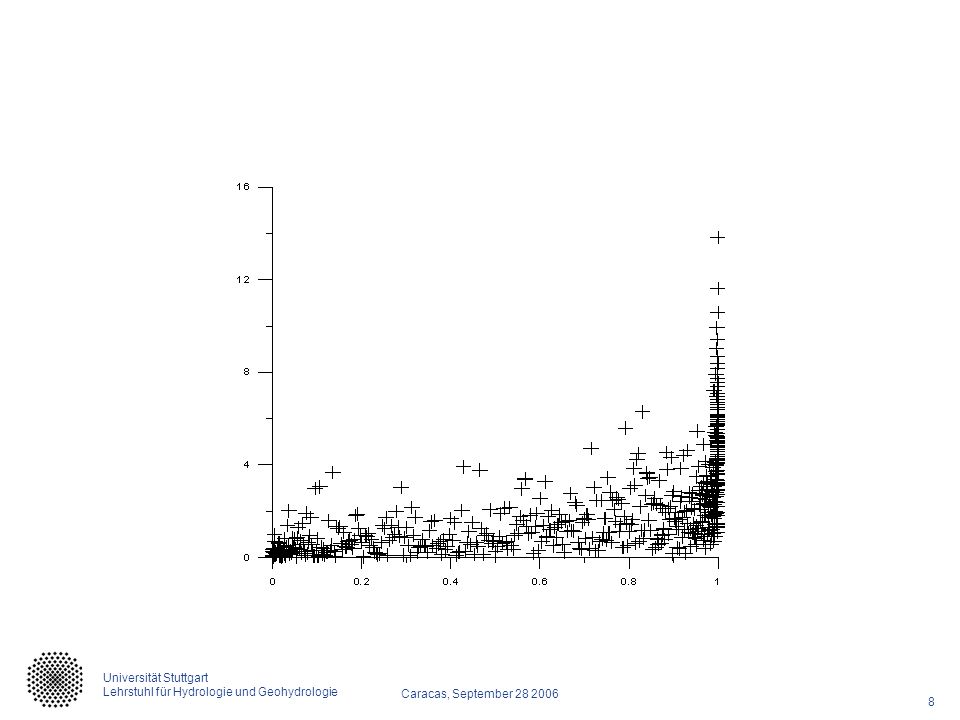
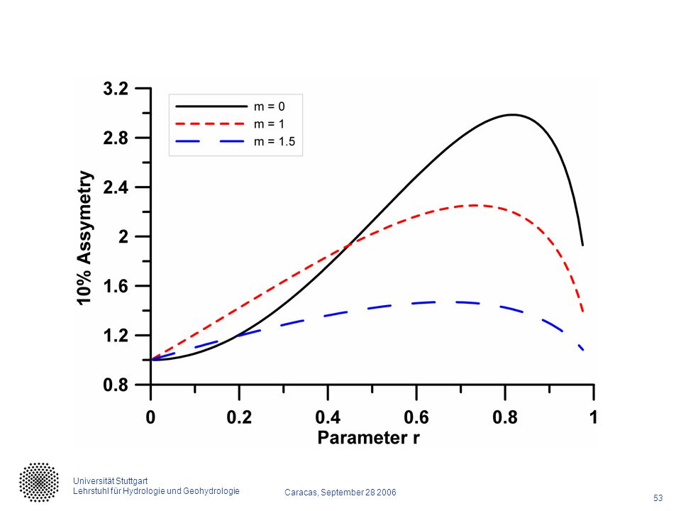
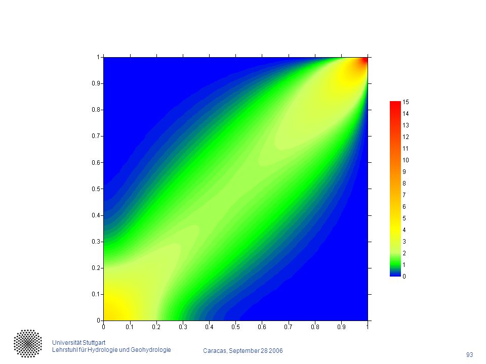
61 Asymmetrie des Zusammenhanges
Hohe Werte zeigen einen anderen Zusammenhang wie die niedrigen

62 Empirische Copuladichten Nitrat pH

63 Radarniederschlag 29. Dezember 2001 8:20-9:20

64

65

66

67

68 Niederschlag Geeignete Copulas finden
Bessere Interpolation (HW relevant) Theoretische Gebietsabminderungsfunktionen Simulationsmodelle mit beliebigen Randverteilungen Realistische Extreme über räumliche und zeitliche Skalen ( Fraktale Modelle)

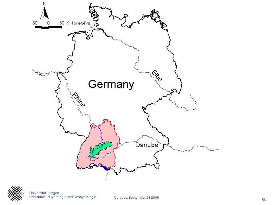
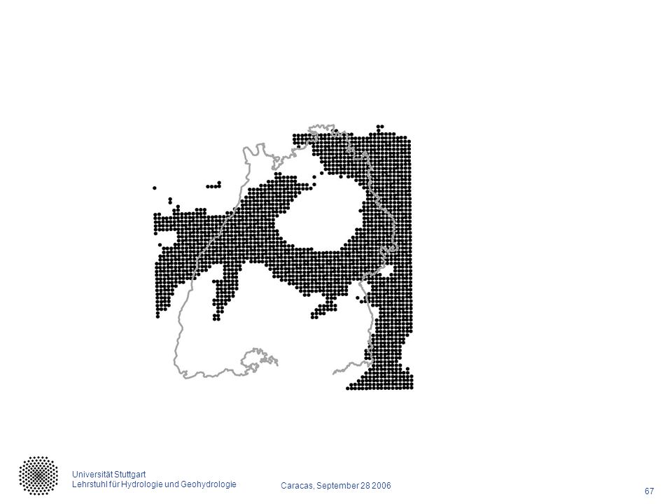
69 Neckar Einzugsgebiet 13 sc! HBV-Model 2.1 Study area and database
The upper Neckar catchment is situated in the SW part of Germany, between the Black Forest to the west and the Schwäbische Alb to the south-east. The southern border of the catchment is the European Watershed, which separates the two big catchments of Danube and Rhine. The river Neckar has its origin at an altitude of 706 m and reaches the outlet of the upper part after 163 km at an altitude of 245 m at Plochingen. With an area of 3995 km2 the catchment represents approximately 28% of the whole Neckar catchment. The highest points lie in the Black Forest (1030 m) and on the Westalb (1014 m), the lowest (245 m) at the outlet in Plochingen. For the Neckar catchment time series of observed daily data is available at a great number of locations. Precipitation data are available at 44 stations inside the catchment and additionally 244 stations in the vicinity. Temperature, snow and wind data are available at 43 stations in and around the catchment. Runoff data are available at 22 gauges in the Upper Neckar catchment. The observation time period for all parameters is from 1961 to 1990.

70

71 Korrelation – Zusammenhang der Extreme (99,5%)

72 Zusammenfassung Zusammenhaänge können mit Copulas beschrieben werden
Viele der Zusammenhänge in der Hydrologie sind asymmetrisch Extreme sind of stärker abhängig als mittlere Korrelation ist hierfür kein gutes Maß

73 Introduction - Modelling
Hydrological modeling is necessary Design Changes Climate change Land use change Unobserved catchments (PUB) Forecasts In combination with Quality Ecology For understanding

74 Introduction - Variability
Variability due to natural conditions Weather Annual cycle Random variability Catchment reaction State Output - discharge

75 The Upper Neckar Catchment
13 sc! HBV-Model 2.1 Study area and database The upper Neckar catchment is situated in the SW part of Germany, between the Black Forest to the west and the Schwäbische Alb to the south-east. The southern border of the catchment is the European Watershed, which separates the two big catchments of Danube and Rhine. The river Neckar has its origin at an altitude of 706 m and reaches the outlet of the upper part after 163 km at an altitude of 245 m at Plochingen. With an area of 3995 km2 the catchment represents approximately 28% of the whole Neckar catchment. The highest points lie in the Black Forest (1030 m) and on the Westalb (1014 m), the lowest (245 m) at the outlet in Plochingen. For the Neckar catchment time series of observed daily data is available at a great number of locations. Precipitation data are available at 44 stations inside the catchment and additionally 244 stations in the vicinity. Temperature, snow and wind data are available at 43 stations in and around the catchment. Runoff data are available at 22 gauges in the Upper Neckar catchment. The observation time period for all parameters is from 1961 to 1990.

76 Dependence between discharge series
Cross correlations (Pearson) Cross rank correlations (Spearman) Copulas

77 Dependence results Cross correlations 0.66 – 0.95 for all pairs
>0.89 for the best pair for each site Cross rank correlations 0.65 – 0.98 for all pairs >0.88 for the best pair for each site

78

79 Dependence structure Dependence between Quantiles instead of Variable values Copula – Dependence separated from the Marginal distributions

80 Copula density of the pair C8 and C9

81 Spatial dependence – 5 km Event 347

82 Spatial dependence – 5 km Event 159

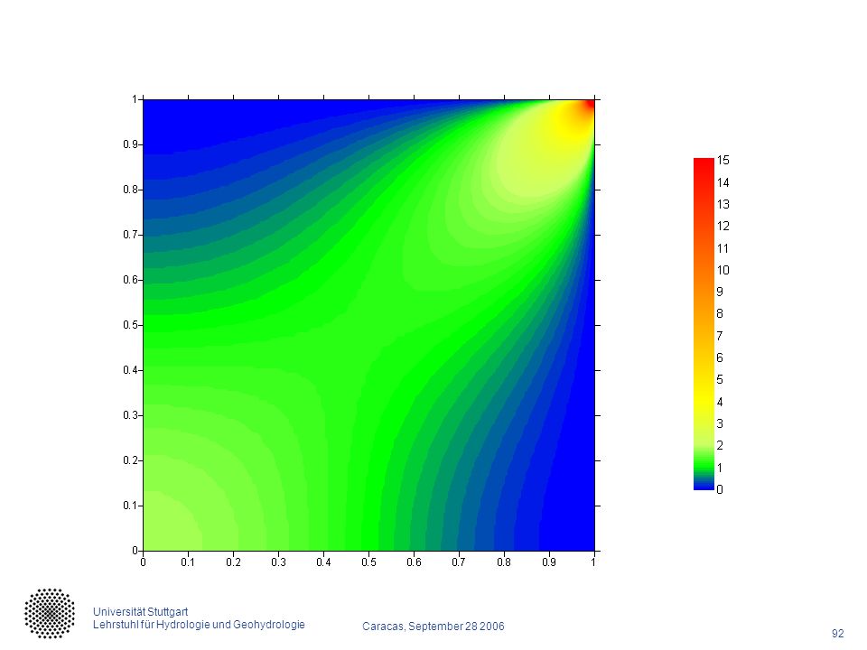
83 Simulation models Multivariate normal copulas
Non Gaussian copulas (non-central chi-square copulas) Correct marginal distribution

84 Copula density of a bivariate non-central chi-square distribution

85 n-dimensional Chi-square copula

86 Summary Hydrological modeling is necessary and difficult
Discharge series are similar Events are different Hydrological models  small differences Spatial resolution is not the answer As mentioned, we are connected globally. The Institute brings learning opportunities to you no matter where you are, to make it convenient for you, in many instances you don’t even need to leave your office… Webinars: These are usually one-hour, online learning opportunities where you can participate free of charge as long as you have Internet access and a phone. Topics focus on products, emerging risks, risk analytics, claims and legal. Webcasting: This expands the concept of webinars to integrate video of the speaker(s) to create a more robust presentation experience. You only need a computer, no phone. Again, accessed at your convenience. Classroom: We offer Practical Thought Leadership; Classes focus on technical training, GE leadership training and customized needs. Most classes can be done in a location convenient for you. Symposiums and Summits: Our Symposiums focus on emerging risks and are held in different areas of the world. We also conduct Global Summits; they have been held in the US, Europe and Asia.  Spatial variability is partly responsible Rainfall variability is “asymmetrical”

87 Interpolation

88 Radar Measurement

89 Future work Compare different sets of downscaled discharge extremes (3 versions) Calculate spatial indices Find appropriate copulas Assess scenario dependent extremes Develop new methodology for spatial extremes

90 Variability of discharge
Distribution of discharge for a single site Depends on the aggregation Skewed distribution Few maxima – due to precipitation (snow melt)

91 Natural Variability Discharge series are similar because of the spatial extent of rainfall events.

92

93

94