Investitionsentscheidungen unter Sicherheit

Präsentation zum Thema: "Investitionsentscheidungen unter Sicherheit"—  Präsentation transkript:

1 Investitionsentscheidungen unter Sicherheit

2 Abnehmender Grenznutzen
Warum kann man Investitionsentscheidungen unabhängig von den Investoren treffen? 1-Perioden-Modell Abnehmender Grenznutzen

3 Abb.2   c  falsch

4 Abb.3 C0 C1

5 Abb.4

6 Abb.5

7 ad. Abb.5: Robinson-Crusoe-Ökonomie: Keine Möglichkeit intertemporären Konsumausgleichs zwischen Individuen. GRS = GRT auf Punkt B Problem: Individuen mit unterschiedlicher Indifferenzkurven wählen andere (opt.) Produktion!

8 Abb.6

9 ad. Abb.6 (Y0,Y1) hat Nutzen U1; man kann durch leihen (und borgen) auf Kapitalmarktlinie Punkt B erreichen mit höherem Nutzen U2. r = Marktzinssatz, zu dem unbeschränkt Geld geliehen oder verliehen wird. (Ergibt sich eigentlich als Lösung eines Gleichgewichtsproblems in einer Ökonomie!) C1* = W0(1+r)-(1+r)C0* bzw. W0(1+r) = W1 C1*=W1-(1+r)C0*

10 Abb.7 A: Anfangszuwendung
C: Weitere Aufgabe von C0 für Produktion B + Leihen von Geld für C0*und C1* D: Aufgabe C0 für C1 zur Maximierung des subj. Nutzens Abb.7

11 Abb.8

12 ad Abb.8: Die Investitionsentscheidung ist von den individuellen Präferenzen unabhängig. GRSi = GRSj = -(1+r) = GRT

13 Annahme: vollkommene Kapitalmärkte vereinfachen vieles - tatsächlich nicht wahr.
Frage: Wie weit gilt Modell? (Analog: Euklidische + sphär. Trigonom.) Investitionsentscheidung: Wieviel konsumieren wir heute nicht zugunsten der Zukunft? Manager sind „Agents of Owner!“ Ziel: Maximiere Nutzen der Eigner: C0 - Dividende C1 - Reinvestition in Prod. Grundannahme: - r ist deterministisch - keine Transaktionskosten - Zukünftige Erträge d. Investition sind mit Sicherheit bekannt

14 Fishers Separations Theorem erlaubt Investitionsentscheidung ohne Kenntnis der Präferenzen (Nutzenfunktion) der Eigner. Problem: Agency-Problem (Nebenleistungen in Aktien - kein Agency-Problem) Nebenleistungen an Manager nur daher beschränkt kontrollierbar.

15 Maximierung des Wohlstands der Eigner W0 (= S0):
(Auszahlungen) ks = Ertrag von Anteilen am Markt (Opportunitätskosten des Kapitals) d.h. Barwert der Erträge des Anteils (Aktie) ist ihr Marktwert (enthält alle Wertsteigerungen!) (ohne Steuer)

16 1) Dividende v. 1 GE und Dividende wächst mit 5 % 2) ks = 10 %
Bsp.: Aktie: 1) Dividende v. 1 GE und Dividende wächst mit 5 % 2) ks = 10 % Gordons Wachstums-Formel! (für ks>g) 5 i=1 5 i=1

17 Für Investitionsrechnung gilt (keine Steuern):
Divt = Ertgt - (Löhne + Material + Dienstleistungen) - Investitionen und  t=0 = Disc. Cash Flow (DCF!) Also: Max. Wohlstand d. Eigner = Max. abgezinsten CF! Modelle für Investitionsentscheidungen = Capital budgeting techniques.

18 Anforderungen an Projektauswahlverfahren:
1) CF sollten verwendet werden. 2) CF sollten zu Opportunitätskosten diskontiert werden. 3) Entscheidungstechn. sollten aus einer Menge sich gegenseitig ausschließender Projekte wählen 4) Wertadditivitätsprinzip: Projekte sollten unabhängig voneinander betrachtet werden können ( V= Vj)

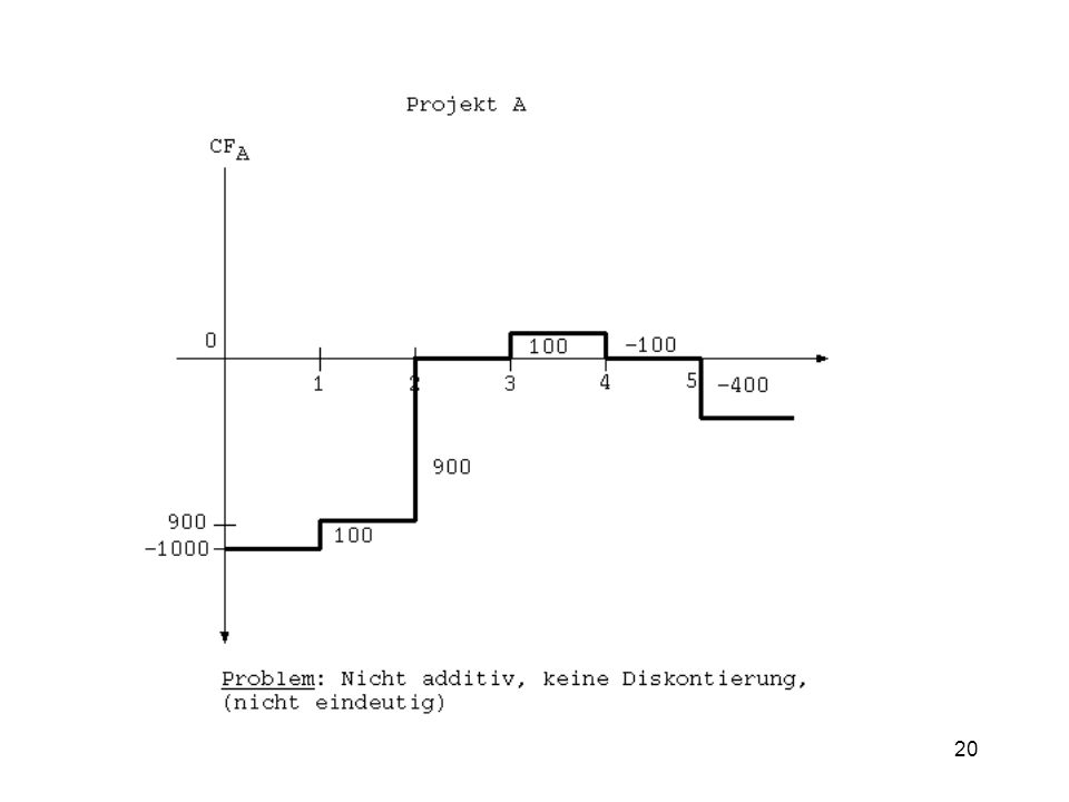
19 Amortisation: Project A, 2 years; Project C, 4 years
Project B, 4 years; Project D, 3 years

20

21 Accounting Rate of Return
Buchhalter. Ertragsrechnung (ROI, RO Assets = ROA): Zuflüsse sind nicht CF sondern After Tax Profits! Annahme: Erträge sind nicht CF, sondern „After Tax Profits“! N i=1 Project A, ARR = -8 % Project C, ARR = 25 % Project B, ARR = 26 % Project D, ARR = 22 % Kritik: no CF no Cashflow no Discounting

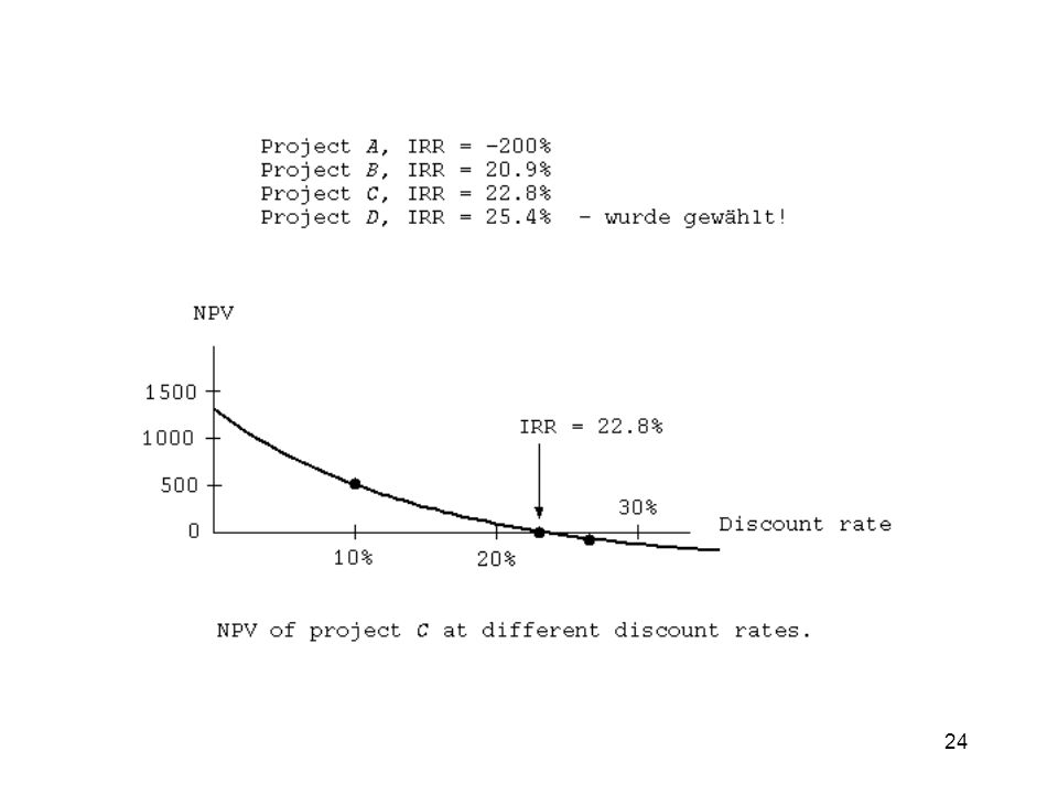
22 Opportunitätskosten des Kapitals
=Barwert N i=1 Opportunitätskosten des Kapitals wurde gewählt! Project A, NPV = ; Project C, NPV = Project B, NPV = ; Project D, NPV = Gegen Intuition: Bei negativem Barwert gilt: weniger Zins „erhöht“ negativen Wert. Bsp: 3 %  1 Mio. neg. Barwert; 10 %  1/2 Mio neg. Barwert.

23 N t=1

24

25 Barwert und interner Zinssatz

26 Kritik: interner Zins a) diskontiert nicht zu den Opportunitätskosten des Kapitals b) nimmt implizit an, der Zeitwert des Geldes sei gleich Interner Zins: Reinvestitionsratenannahme (Verletzt somit auch Fishers Separation Theorem) c) Kann gezeigt werden, verletzt Wertadditivitätsprinzip (Prinzip: Wert des Ganzen ist gleich Summe der Teile) d) Mehrfacher Interner Zinsfuß möglich Folge: DCF ist das einzig vertretbare Verfahren zur Wahl von Projekten zur Maximierung des Wohlstands des Eigners.

27 *Percentages shown are yes divided by yes + no, multiplied by 100.
Klammer,T., „Empirical Evidence of the Adoption of Sophisticated Capital Budgeting Techniques,“ reprinted from The Journal of Business. July 1972, 393.

28 , 

29

30 Investitionsentscheidungen unter Unsicherheit

31 St. Petersburg Paradoxon:
Münzwurf: Wenn das 1.Mal Wappen nach N Würfen auftritt, dann wird bezahlt 2N. Erwarteter Wert:  2i = Ergebnis: Das Spiel ist seinen Erwartungswert nicht wert! Beweis: Introspektion LÖSUNG: Individuen interessiert nicht der Geldwert, es interessiert der subjektive Nutzen des Geldwertes: Grenzertrag von Geldeinkommen nimmt mit Zunahme des Einkommens ab! 1 2i {i}

32 Wert des Spiels für Individuum U(x) = log2 (n)
Erwarteter Nutzen: Wert des Spiels für Individuum U(x) = log2 (n) {i} {i} Hypothese: Individuen wählen in Unsicherheit nach erwarteten Nutzen. Individuen verwenden Bayes Entscheidungsregel! (Subjektive Wahrscheinlichkeit + erwarteter Nutzen  N-M-Axiome rat. Verhaltens Übereinstimmung) Unter den Voraussetzungen des N-M-Axiomensystems kann man eine Nutzenfunktion u: W  R1 konstruieren, die effizienter verwendbar ist als ein ordinaler Nutzenindex:

33 V.Neumann - Morgenstern
AXIOMENSYSTEM von V.Neumann - Morgenstern N1. Auf der Menge der Lotterien W existiert eine schwache Präferenzrelation „< „, es sei „<„ die zur Relation „ < „ gehörige strikte Präferenz. N2. Es seien P, Q, R Lotterien und 0<1, dann gilt P < Q   P + (1- )R < Q + (1- )R N3. P,Q,R seien Lotterien und P<Q<R, dann gibt es Zahlen ,  mit 0<  <1 und 0< <1 , so daß gilt: P + (1- )R <Q<  P + (1-  )R. ~ ~

34 A) Ordnungstreue (Monotonie): P< Q  U(P)  U(Q) B) Linearität:
Erwartungsnutzen Definition: Eine Funktion U:W  R1 heißt Erwartungsnutzen, wenn sie folgende Eigenschaften erfüllt: A) Ordnungstreue (Monotonie): P< Q  U(P)  U(Q) B) Linearität: U(1P1+ 2P K = 1U(P1) + 2U(P2)+...+ KU(PK) C) Eindeutigkeit bis auf positiv-lineare Transformationen: seien u,v zwei Funktionen, welche A) und B) erfüllen, dann gilt: U(P) = AV (P) + B mit A >0 I ~

35 Hauptsatz der kardinalen Nutzentheorie
Auf einer Menge von Lotterien W, welche 1. die Axiome von v.Neumann - Morgenstern erfüllen und 2. in der es mindestens ein paar P, Q mit P< Q gibt existiert ein Erwartungsnutzen: Beweisidee: Setze u(P) = 0 und u(Q) = 1 A) Für P<R<Q kann man aus Axiomen folgern: Es gibt ein eindeutiges  (  (0,1)), so dass R~ P+(1- )Q gilt. Hieraus: u(R) = 1-  (R heißt Sicherheitsäquivalent von P+(1- )Q analog: R<P<Q und P<Q<R

36 Є ist meist eine Menge von monetären Konsequenzen (homogenes Gut).
Bernoulli-Prinzip: Є ist meist eine Menge von monetären Konsequenzen (homogenes Gut). uo: R1R1 mit uo (x) = u( ) (oft einfach u(x)) Ergebnis des Hauptsatzes: u(P) = E(u(x)) für P Є W Beispiel: x1 x2 P = p 1-p Zwei Zufallsvariable: u(x) (Nutzen u(xi) mit Wahrscheinl. pi) x (Geldbetrag xi mit Wahrscheinl. pi) Nach Hauptsatz gilt: u(P) = p u(x1) + (1-p) u(x2) (=E(u(x))) Meist gilt zudem u(P)  E(x) außer wenn u(x) linear Э x [ ] 1

37 Nutzenfunktion: Problem des Sicherheitsäquivalents: Finde einen Wert ξ derart, dass z.B. (Zweipunktverteilung) gilt: u(ξ) = u(P) = p(u(x1)) + (1-p)u(x2) (P Є W) = E(U(K))  u-1(E(u(x)) = ξ

38 Bsp: konvexe Nutzenfunktion (Risikofreudigkeit)
u(x) = x²/10 : Fixpunkte u(x) : x = 0 x = 10 Ermittele für u(x) das Sicherheitsäquivalent von Lotterie: u(x2)-u(x1) Also: ξ > E(x) ξ  15,

39 Experimentelle Ermittlung von ξ:
Man ermittle ξ, so daß A1 ~ A2; d.h. p 1-p ~ p p ξ ξ x1 x2 , also U{ξ} = p u(ξ) + (1-p) u(ξ) = p u (x1) + (1-p) u(x2) also 10 20 = P u(ξ) = E (u(X)) ½ ½

40 Bsp.: p= 0,5; Bekannte Nutzenfunktion:
E(x) = 10 * 0, * 0,5 = 15 E(U(x)) = 40 * 0, * 0,5 = 25 = u(ξ) U(E(X)) = = 22,5 ξ =  25 x 10  15,8 (=u-1(u(ξ))) E(U(X)) = 25 u-1(E(U(x))) = ξ > E(X)  Risikofreude (U-1(U(E(X)))) = E(X) ξ < E(X)  Risikoaversion 15² 10

41 1-p p u(x2)-u(x1) Also: ξ < E(x) ξ

42

43 Risikoaversion und Risikoaversionsmasse
Kard. Nutzenfunktion ist unter gewissen rationalen Voraussetzungen aus Präferenzrelation  bildbar. Bsp.: a  b 1-  Wahrscheinlichkeit Risikoprämie: Maximum an Wohlstand, den ein Individuum aufgeben würde, um Risiko zu vermeiden.

44 Markowitz´sche Prämie: E(W) - ξ (von W abhängig)
Bsp.: Es gelten U(W) = ln (W) (logarithm. Nutzenfunktion) ξ ξ

45 Indifference curves for a risk-averse investor.
σ Indifference curves for a risk-averse investor. Verteilung der Erträge: gemeinsam normal verteilt + Risikoaversion (multivariat normal), dann wird erwarteter Nutzen maximiert durch beste Wahl der Kombinationen aus (µ, σ).

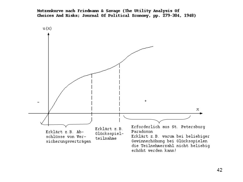
46 Nutzentheorie: Wenig emp. Test; Psychologie: z.B.: Kahneman & Trevsky Survival Frame Mortality Signifikante Differenz Savage Bsp. (intuitiv intransitiv) Resultat: Eher nicht realistisch Krebsbehandlung Ferschl

47 Risiko und Ertrag einer Investition
Anfangsinvestition = I Wohlstand zu Ende Investitionsperiode = W Zins: R = W = (1+R) I I = (1+R)-1 W W-I I

48 Problem: Wie sollen Investitionsbeträge investiert werden! (In jedes mögliche Projekt) Markowitz Ansatz: Betrachte Trade-off von Risiko und Ertrag Risiko: Fast immer mit VARIANZ modell.

49 Hauptidee: Ertrag von Investition ist ZV
Wie investiert man: Investiere alles in das Projekt mit höchstem E(W). (erwartetem Ertrag). Investoren machen das nicht, da risikoavers. Diversifikation reduziert Risiko!

50 Beispiel: Portfolio aus 2 Investitionen (X,Y) mit Ertrag (R): RP = aX + bY mit b= 1-a E(RP) = a E(x) + b E(Y) a² (RP) = a²²x + b²²y 2ab xy

51 Negative Kovarianz: Gewinn in X  Verlust in Y Investition partiell „gehedged“ geringeres Risiko E(X) = 10 % E (Y) = 8 % ²x = 0,0076 ²y = 0,00708 xy = -0,0024 ρxy = -0,33 = xy / x y

52 ²RP = a² ²x + (1-a)² ²y + 2a (1-a) ρxy x y
=Optimum P=aX+(1-a)Y

53    in %  in % The portfolio return mean and standard deviation as a function of the percentage invested in risky asset X.

54   Leerverkauf von 50 % in X und Kauf von 150 % in Y: E(RP) = -0.5 E(X) E(Y) = 0,07  RP = 0,1464

55 Minimum Varianz Portfolio
²Rρ = a² ²x + (1-a) ²y + 2a (1-a) ρxy x y Minimale Varianz durch: Bsp: a* = 0,487 Opt. Portfolio: E(Rp) = 8,974 % Rp = 4,956 %

56 Perfectly Correlated ρ = -1 X = 1,037Y + 1,703 ρxy = 1 a* = 0,49...
E(Rpa*) = 8,98.. %  (Rpa*) = 0 % X = 1,037Y + 1,703 ρxy = 1

57 MINIMUM VARIANCE OPPORTUNITY SET
Ort aller Risiko-Ertrags-Kombinationen von Portfeuilles risikoreicher Anlagen die minimale Varianz für gegebenen Ertrag R aufweisen. ρ xy=-1 ρxy=0,1 ρxy= -0,33  ρxy= 1  ρxy = -1; ²Rp = (ax - (1-a)y )² Rp = +/- (ax + (1-a)y )

58 Wahl des optimalen Portfeuilles
1) 2 risikoreiche Anlagen Robinson-Crusoe-Fall: keine Tauschmöglichkeit R-C-Portfeuille: Subjektive Grenzrate d. Subst. von Risiko +Ertrag = Objektive Grenzrate d. Transformation (M-Var.-Opt. Set) und Risiko + Ertrag

59 MRS=MRT E(Rρ) Rρ Optimal portfolio choice for a risk-averse investor and two risky assets.

60 Problem: Auch bei homogenen Erwartungen verschiedene opt
Problem: Auch bei homogenen Erwartungen verschiedene opt. Portfeuilles wegen individueller Nutzenfunktion E(Rρ) E(R) of MIN Effiziente Menge: Nicht dominiertes Portfeuilles Rρ MIN (R)

61 Sonderfall: ρxy = -1 oder +1
Efficient set. The efficient set is the set of mean-variance choices from the investment opportunity set where for a given variance (or standard deviation) no other investment opportunity offers a higher mean return (previous page). Sonderfall: ρxy = -1 oder +1 Eff. Menge bei ρxy = -1 E(Rp) ρxy = +1 Rp

62 Problem: Auffinden der µ-- Opportunity-Menge
Lösung folgender Programmierprobleme: PrProb. 1: MIN ² (Rp) unter E(Rp) = Konstant PrProb. 2: MAX E(Rp) unter ² (Rp) = Konstant Da die Zielfunktion z.B. in PrProbl.1 gleich MIN {² (Rp) = (a² ²x +(1-a) ²y +2a(1-a) ρxy x y)} liegt quadrat. Programmierproblem vor. (Entscheidungsvariable: Finde a!) Markowitz (1959) hat das Entscheidungsproblem des Investors erstmals dieser Art definiert und gezeigt, dass der Investornutzen so maximiert wird.

63 Risikofreier Zinssatz
What if there is a risk free asset available? Risk free asset = one with a certain return. Corporations have default (=Bankrott) risk, so we must consider treasury securities. Suppose we have a 1 year holding period: - 10 year T-note has interest rate risk - 90 day T-bill has reinvestment rate risk. Thus, the only risk-free asset is a treasury security with a maturity that matches the length of the investor´s holding period. (comments: -there should be no coupons (reinvestment risk) - there is still inflation risk!)

64 Effiziente Menge mit einer Investition mit Risiko und einer risikofreien Anlage Rf
E(Rp) a > 1 E(X) 0  α  1 Rƒ hat Varianz Ø. Es gilt dann: E(Rp) = a E(X) + (1-a) Rƒ ² (Rp) = a² x² Borrowing = Leerverkauf der risikofreien An- lage Lending Rƒ (Rp) (X)

65 Risiko und Ertrag eines Portfeuilles mit mehreren Investitionsmöglichkeiten
bzw. = R´W ² Rp = W´ W ( = Kovarianzmatrix) übrigens: cov (Rp1,Rp2)=Wp1  Wp2 oder cov (RA1,Rp) = ( )  Wp P = Portfolio A = Anlage

66  =

67 E(Rp) I z.b. (Rp)

68 Eine risikofreie und N Anlagen mit Risiko
B ungünstiger als M Rƒ 

69 Einführung von vollk. Kapitalmarkt : Wirkung
Jeder Investor ist mindestens ebenso gut (II) wenn nicht besser dran. 

70 Marginal Rate of Substitution = Marginal Rate of Transformation
Two-fund separation. Each investor will have a utility-maximizing portfolio that is a combination of the risk-free asset and a portfolio (or fund) of risky assets that is determined by the line drawn from the risk-free rate of return tangent to the investor´s efficient set of risky assets. (Tobin) Capital market line (CML). If investors have homogeneous beliefs, then they all have the same linear efficient set called the capital market line. Jedes opt. Portfeuille P liegt dort mit dem Ertrag E(Rp)

71 CAPM (Capital Asset Pricing Model)
CAPM is the intellectual basis for much of the current investment industry. Markowitz - How should an investor invest? (normative) CAPM - What will happen if everyone invests this way?

72 Assumptions: 1) Investors are Markowitz efficient diversifiers who delineate and seek the efficient frontier a) they look at expected returns and variances b) they are never satiated c) they are risk averse d) assets are infinitely divisible e) taxes and transaction costs are irrelevant f) there is a risk free rate at which an investor may either borrow or lend

73 2) All investors have the same one-period horizon
3) Risk free rate is the same for all investors 4) Information is freely and instantly available 5) Investors have homogeneous expectations How will assets be priced under these assumptions, assuming the markets are in equilibrium? Specifically, what is the equilibrium relationship between a security´s risk and return?

74 Implications of CAPM assumptions:
All investors will choose the same tangency portfolio. This follows from the separation theorem and the homogeneous expectations assumption. E (Rp) M rƒ p

75 What is M? 1) Every security must be represented (if no one is buying asset T, its price will fall, hence its expected returns will rise) 2) The number of shares demanded of each security will equal the number of shares outstanding, and the proportion of each asset will be its relative market value. w(A) = market value of asset A / total market value of all assets (market value = market clearing price; we assume equilibrium) If everybody has less than w(A), there will be shares outstanding,  the price will go down If everybody wants more than w(A), there will be not enough shares to go around,  price will go up.

76 Thus M is the market portfolio!
Example: S&P500 Index, A market cap weighted average of the market prices of 500 large stocks. A proxy for the stock segment of the market portfolio. Also used: NYSE-Index Implications for CAPM: Since each investor holds the market portfolio (in conjunction with borrowing or lending at the risk free rate), investors are concerned with the risk of the market portfolio. What is the relevant measure of risk of a security? - it is not the standard deviation - it is the covariance with the market portfolio To see this, compute the variance of the market portfolio

77 NOTATION: M= w1A1 + w2A wNAN Ai = the ith asset ri = the return on the ith asset i,j = COV(ri,rj) LEMMA: The covariance of an asset with a weighted sum is the weighted sum of the covariances COV(ri,rM) = COV (ri,  wjrj) =  wjCOV(ri,rj) oder ²M = WW = W (W) = wi iM

78 Thus the risk of the market portfolio is a weighted sum of the covariances of each asset with the market portfolio. Normalizing these covariances by the variance of M, we have the definition of Beta.

79 BETA βi = σiM / σM² The relevant measure of the risk of an asset in CAPM Für I = M gilt: βM = 1

80 CAPITAL ASSET PRICING MODEL:
E (ri) = rf + (E(rM) - rf) βi where βi = COV (ri, rM) / σM² Thus a security´s expected return is positively and linearly related to its Beta (every security)

81 (Security Market Line) Every Security plots on this
SML: (Security Market Line) Every Security plots on this line (auch jene, die nicht im Portf. des eff. Randes liegen) z.B. AI CML: (Capital Market Line) SML M rM rƒ AI β rp Slope = E (rM) - rƒ σM M E (rM) AI rƒ σp σM

82 Derivation of CAPM: Consider P = wiAI + (I-wi) M 1) Find E (rp) , σp 2) Find d E(rp)/ dwi d σp / dwi 3) Evaluate at M (wi = 0) Da I bereits in M ist , ist wI in Gleichgewicht 0. 4) Set equal to E (rM) - rf , slope of CML σM 5) Result: E (rI) = rf + (E(rM) - rf) COV(rI,M) = rf + (E(rM) - rf) βI σM²

83 Appendix Ableitung CAPM 1) Existiert Gleichgewicht  Angebot = Nachfrage ergo : wi = Marktwert von Anteil I-Projekt Marktwert aller Projekte 2) Für ein Portfeuille P mit wI in I und (1-wI) in M gilt: E(Rp) = wI E (rI) + (1-wI) E(rM) σRp = (wI² σI² + (1-wI)² σM² + 2wI (1-wI) σIM)1/2 Weiters gilt: d E(Rp) / da = E(rI) - E(rM) d σRp / da = 1/2(wI² σI² + (1-wI)² σM² + 2wI (1- wI) σIM)1/2 x (2wI σI²-2 σ²M- 2wI σM²+ 2 σIM +4wI σIM)

84 Da das Marktportfeuille M bereits I enthält, folgt wI =0 in Gleichgewicht; daher:
d E(rp) /da = d E(rp) = E(rI) - E(rM) d σrp / da wI=0 d σrp wI= σ IM - σ ²M σ M Da für die CML das Portfeuille auch in Gleichgewicht ist und Steigung E(rM) - rf aufweist, folgt aus: E(rM) - rf = E(rI) - E(rM) σM (σIM - σ²) / σM oder E(rI) = rf + ( E(rM)- rf) = rf + λ βI σIM σ²M

85 CAPM applies to both active and passive portfolio management
passive:buy S&P500, and treasuries active: (=tactical asset allocation = market timing) forecast asset prices, if they are underpriced or overpriced buy or sell accordingly. E(r) A=4% Schätzung mit lin. Regression:  j E(rj) = aj + j RM + j (= unkorrelierte ZV) σ²j= ² σ²m+ σ²=system.Risiko + unsyst.Risiko B=3% rf 

86

87 Man kann zeigen: CAPM: W1 βM = (β1 , β βn ) W2 .. WN N wenn E(rM) =  wi E(ri) i=1

88 Summary: CAPM is the grand-daddy of asset pricing models.
- there is not much evidence to substantiate its validity - there is debate as to whether it is even testable, what is the market portfolio? S&P500 used as proxy, to estimate betas. - it has generated much useful empirical information CAPM has many children: Extensions, alternative models. - relax assumption that lending rate = Borrowing Rate - heterogeneous expectations; each investor has unique efficient set and tangency portfolio - investors also concerned with liquidity (not just risk and return)

89 Weiterentwicklung: Arbitrage Pricing Theory = APT (Ross 1976) statt 1-Faktoren Modell (CAPM) Faktor = rM = Ertrag des Marktportfolio) n-Faktoren Modell

90 ARBITRAGE A METHOD OF VALUATION The law of one price: A security can have only one price Arbitrage = riskless profit due to price discrepancies. The Hypothesis of no-arbitrage possibilities allows the valuation of derivative securities. Example: Futures contract on a security that pays no dividends How much is it worth? F* = Fair Price F0 = Futures price now S0 = Stock price now FT = Futures price at expiration ST = Stock price at expiration r = riskless rate F* = S0 (1 + r) The answer has nothing to do with expectations!

91 Futurespreis und Periode muß gleich F
Futurespreis und Periode muß gleich F* = S0 (1+r) sein, sonst risikoloser Gewinn! Reason: Suppose F0 > S0 (1+r) Sell the futures; must hedge borrow S0 dollars and buy the stock At Expiration, liquidate: Futures position: F0 - FT Stock Position: ST - S0 (1+r) But FT = ST (F0 - FT ) + (ST - S0 (1+r)) = F0 - S0 (1+r) >0 Riskless profit! Bet the farm! Result: Heavy futures selling will force F0 down, until the ARB disappears.

92 Conversely: Suppose F0 < S0 (1+r)
Buy the futures; must hedge sell the stock, invest the S0 dollars At Expiration, liquidate: Futures position: FT - F0 Stock Position: S0 (1+r) - ST But FT = ST (FT - F0) + (S0 (1+r) - ST) = S0 (1+r) - F0 > 0 Riskless profit! Bet the farm! Result: Heavy stock selling will force F0 down, until the ARB disappears.

93 Key ingredients of this analysis:
Arbitrage opportunities cannot persist - Arbitrageurs are like policemen who enforce the law of one price ASSUMPTIONS: Short selling no problem No Transaction costs Borrowing rate = Lending rate Also the above example was quite simplified: 1) The industry uses continuous compounding models: F* = S0 ert 2) The instrument might throw off known amount of cash F* = (S0 - I) ert I = present value of cash flows 3) Instrument might generate dividends F* = S0exp[(r-d)T]

94 OPTIONEN (Aktien) (1973 mit CBOE eingeführt) Kaufoption (CALL): Vertrag, der erlaubt, eine Aktie der Gesellschaft zu einem festen Preis (Ausübungspreis) zu einem gewissen Zeitpunkt (oder innerhalb einer gewissen Frist) zu kaufen. Kaufoptionen können 1) gekauft oder 2) verkauft werden.

95 Verkaufoptionen (PUT): Erlauben Inhaber des Vertrages zu verkaufen zu späterem Zeitpunkt (oder innerhalb einer Frist) zu festem Preis. Sie können: 1) gekauft oder 2) verkauft werden

96 Auszug: Chicago Board Listed Options Quotations (4. Oktober 1977)
C=ƒ(S,X, σ²,T,rƒ) 12 3/4 Erhöht die Wahrscheinlichk. W(S>X); Ertrag nur von Verteilungende.

97 Payoffs von CALL-Option
Cer ƒT -Cer ƒT W S Payoffs von CALL-Option W = Änderungen von Wohlstand S = Änderungen von S

98 Europäische Kaufoption in einer „alternativen“ Welt.
S = $ = the stock price, q = .5 = the probability the stock price will move upward, 1+rƒ = 1.1 = one plus the risk-free rate of interest, u = 1.2 = the multiplicative upward movement in the stock price (u > 1 + rƒ > 1), d = .67 = the mulitplicative downward movement in the stock price (d < 1 < 1 + rƒ )

99 Wert der Option c? uS = 24 dS = 13,40 X =

100 Konstruktion eines risikofreien sicheren Endvermögens:
Ausgangspunkt: Wir kaufen 1 Aktie um S und verkaufen m Kaufoptionen um c m. Nach einer Periode soll gelten: uS - mcu = dS - mcd d.h. es muß gelten:

101 in unserem Beispiel gilt:

102 Da das sichere Endvermögen risikolos war, muß gelten:
(1+rf) (S-mc) = uS - mcu oder:

103 C=(pcu + (1-p) cd) / (1+rf)
c= ( x x 0) / 1.1 =

104 Es gilt: 0<p<1 und p wird als Hedging-Wahrscheinlichkeit bezeichnet!

105 Cun dT-n = max (0, un dT-n S-X)
Wir behandeln dies wie eine Stichprobe aus alternativ verteilter Gesamtheit mit p; es gilt für T Perioden für die Option: Cun dT-n = max (0, un dT-n S-X) Also: T n=0

106 und p= (1+rf) - d sowie p‘ = u p
Durch Umformung kann man schreiben:  und p= (1+rf) - d sowie p‘ = u p u-d (1+rf) und a =  ln (X/Sd“) / ln (u/d) 

107 Cox, Ross und Rubinstein (1979)
Es gilt mit n   B(na / T,p´)  N (d1) und B(na / T,p)  N (d2) d.h. mit n   gilt die Black-Scholes-Formel (1973): c = S N (d1) - Xe -rfT N (d2) d2 = d1 -  T

108 Gilt nicht für amerikanische Optionen!
Gilt für: Optionen auf Anleihen, Indexen Optionen auf Futures Optionen auf Zinssätze und Wechselkurse Optionen auf SWAPS usw. Optionen, immer dann wenn Flexibilität vorhanden  REAL OPTIONS! Aktien: Optionen hängen von einer zugrundeliegenden Zufallsvariablen ab: Vermögenswert = Aktie

109 Wir verwenden kontinuierlichen Zinseszins:
B = Sn = P0 (1+r)n jährlich Sn = P0 (1+r 2)2n halbjährlich Sn = P0 (1+rm)mn m-Verzinsungs- zeitpunkte pro Perioden wegen Sn = P0 ((1+ rm) r/m)rt für m´= m/r erhält man Sn = P0 ((1+1 m´)m´ )rt

110 Geht m nach , so geht m´nach  und man erhält wegen:
Sn = P0 ert für t0 bzw.: P0 = Sn e-rt

111 Sicheres Endvermögen: X daher diskontierbar mit rƒ
Bewertung des PUT im allgemein komplitzierten Einfacher mit: PUT-CALL-Parity (nur europ. PUT (d.h. ohne Dividende und auszuüben nur zu Periodenende)) Portfeuille: 1 Aktie - KAUF 1 Put-Option - KAUF 1 CALL-Option - VERKAUF X= Ausübungspreis T= Laufzeit Sicheres Endvermögen: X daher diskontierbar mit rƒ

112 Diskrete Abzinsung: (rƒ = Zins für Periode) Für S0 = X gilt: C0 - P0 = rƒ S0 / (1 + rƒ ) > 0 Stetig: C0 - P0 = S0 - Xe- rƒt

113 Strategische Aspekte und IT-Einsatz
Barwertanalyse hat u.a. den Mangel der Nichtbeachtung strategischer Aspekte: Beispiel:IT-Investition (2 Umweltzustände nach 1 Jahr) DM 200 DM 80 0.5 DM 118 Projekt nicht mit Geschäftsrisiko des Unternehmens selbst hoch korreliert, daher vergleichbares „Gut“ zu suchen, mit demselben Ertrag: S=DM 28 uS= x 28 = 50 dS= x 28 = 20

114 Lineares Vielfaches von Projekt, daher gilt für Zins
oder r = 25 % 0.5 200 80 Alternative: 1 Periode warten Investieren ? Warten BW = -6 BW = ? (Investitionskosten steigen mit 8 %) ja nein BW = 0 0.5 max { x 1.08,0} = 72.56 max { x 1.08,0} = 0

115 Suche replizierendes Portfeuille am Markt!
Wir kombinieren unser korreliertes Gut S mit dem risikolosen Entlehnen von B DM (m = Anzahl der Anteile von S, B = Anzahl der risikolosen Anteile): Wir erhalten das Gleichungssystem m x (uS) - (1 + rƒ ) B = 72.56 m x (dS) - (1 + rƒ ) B = 0 und für uS = 50 und dS = 20 mit rƒ = 0.08: B= und m = 2.42 Aktien Da dieses Portfeuille den gleichen Ertrag hat, wissen wir dessen Wert: mS - B = 2.42 x = 22.97 Der Wert der Option auf Verzögerung ist also Projektbarwert (-6) = 28.97

116 Andere reale Optionen:
Option auf Projektabbruch (mit Teilerlösen) (Put-Option) Option auf Projektbeginn - oder -entwicklungsverzögerung Option auf Projekterweiterung Option auf Projektreduktion u.a.m. Viele hiervon relevant für IS- und IT-Investitionen bisher praktisch nicht explizit berücksichtigt. (Vgl. A. Dixit, R. Pindyck, Investment under uncertainty, Proctor Univ. Press, 1994 und insbesondere zum Zusammenhang von Entscheidungsbaumanalyse und reale Optionen: Nau, R.F. und Smith, J.E., Valuing Risky Projects: Option Pricing Theory and Decision Analysis, Management Science, Vl. 41, No. 5, pp (1995)) Copeland, T., Real Options, Texere, 2001.