Präsentation herunterladen
Die Präsentation wird geladen. Bitte warten

1
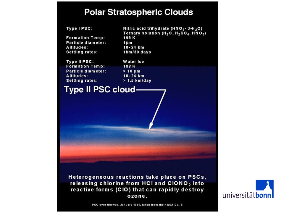
Stratospheric Ozone polar stratospheric clouds
Image: polar stratospheric clouds

2
Die Ozonproblematik Quelle: US EPA (

3
Stratosphärische Ozonschicht schützt vor UV Strahlung
UV-B

4
Stratosphärische Ozonschicht schützt vor UV Strahlung
UV-A: nm UV-B: nm UV-B UV-A

5
Brief history of stratospheric ozone (1)
1881 Hartley identifies ozone as main cause for cutoff of solar spectrum at 300 nm 1921 Fabry and Buisson obtain first reliable measurement of overhead column ozone 1918 Strutt measured tropospheric „column“ with „40 ppb or less“ bulk of ozone in stratosphere 1926 Dobson and Harrison measure latitudinal distribution of total ozone 1930 Chapman theory; Schumacher measured rate coefficients Götz identified an ozone layer and located maximum near 22 km between 1934 and the 1970s, people were convinced that the Chapman theory is correct; the obvious disagreement of the latitudinal distribution and the seasonal cycle were thought to be uncertainties in transport

6
Brief history of stratospheric ozone (2)
1960 McGrath and Norris discover OH production and propose catalytic ozone destruction cycle 1971 Crutzen and Johnston discover NOx cycle 1974 Molina and Rowland recognize impact of man-made chlorofluoromethanes 1985 Farman discovers Antarctic ozone hole Montreal protocol 1995 Nobel prize for Crutzen, Molina, and Rowland Ozone reports at WMO:

7
Verteilung von Ozon

8
Ozon-Vertikalprofile in der Nordhemisphäre
Januar April Dütsch, 1974

9
Merdionalschnitt der Ozonverteilung in nb
February May August November 1 nb = 10(-4) Pa = 0.1 mPa Dütsch, 1974
 Pa = 0.1 mPa. Dütsch,")
10
Merdionalschnitt der Ozonverteilung in ppm
April June October December 1 nb = 10(-4) Pa = 0.1 mPa Dütsch, 1974
 Pa = 0.1 mPa. Dütsch,")
11
Dobson Units 1 DU entspricht der Menge Ozon in der Gesamtsäule, die bei Normaldruck (1015 hPa) und 0C in eine Höhe von 0.01 mm passen würde. Typischer Wert für die Ozonsäulendichte: 300 DU Herleitung 1 DU = 2.69e16 molec cm-2 unmittelbar aus Teilchenzahldichte ideales Gas (2.69e19 molec cm-3) mit h=0.01 mm= cm oder etwas umständlicher: aus molec cm-2 = g/cm2 * mole/g * molec/mole folgt coldens = rho*h*Na/molmass(O3) und wegen rho=p*molmass(O3)/(R*T): coldens = p*h*Na/(R*T) : print "%e" % ( /8.314/273.15*1.e-5* e23) e [ in molec m-2 !] 1 DU = 2.691016 molec. cm-2
 mit h=0.01 mm= cm. oder etwas umständlicher: aus molec cm-2 = g/cm2 * mole/g * molec/mole folgt. coldens = rho*h*Na/molmass(O3) und wegen rho=p*molmass(O3)/(R*T): coldens = p*h*Na/(R*T) : print %e % ( /8.314/273.15*1.e-5* e23) e+20 [ in molec m-2 !] 1 DU = 2.691016 molec. cm-2.")
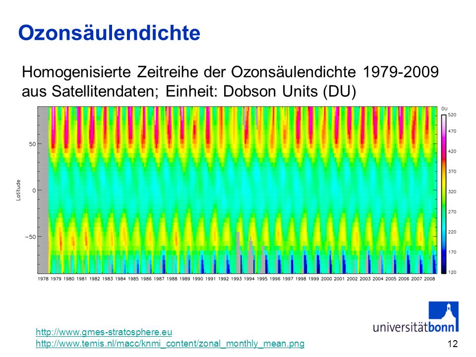
12
Ozonsäulendichte Homogenisierte Zeitreihe der Ozonsäulendichte aus Satellitendaten; Einheit: Dobson Units (DU)
13
Ozonsäulendichte Jan Jul

14
Der Chapman Zyklus (1) (1) O2 + h O + O (2) O + O2 + M O3 + M
 (1) O2 + h O + O (2) O + O2 + M O3 + M")
15
Der Chapman Zyklus (2) (1) O2 + h O + O (2) O + O2 + M O3 + M
Bilanzgleichung für Ozonkonzentration: Im Gleichgewicht:

16
Der Chapman Zyklus (3) P L
Verlustterm L fast immer linear von der Konzentration (hier O3) abhängig. Daher: bzw.:
 abhängig. Daher: bzw.:")
17
Lebensdauer (1) Allgemeine Masse-Bilanzgleichung in einem Teilvolumen der Atmosphäre: Definition der Verweildauer: Bei Annahme des Gleichgewichts ("steady state") gilt ebenfalls: nach Seinfeld/Pandis Bezieht man die gesamte Atmosphäre als Reservoir ein, dann folgt: Dieses ist die Lebensdauer
 gilt ebenfalls: nach Seinfeld/Pandis. Bezieht man die gesamte Atmosphäre als Reservoir ein, dann folgt: Dieses ist die Lebensdauer.")
18
Lebensdauer (2) Wenn der Verlust erster Ordnung ist (also proportional zu Q): Bei mehreren Verlustprozessen gilt: bzw.: nach Seinfeld/Pandis

19
Lebensdauer (3) Bei inhomogener Konzentrationsverteilung bzw. nicht-konstanter Reaktionsrate (also im Regelfall), muss integriert werden: nach Seinfeld/Pandis

20
Ozonverteilung aus dem Chapman-Zyklus
Konzentration Lebensdauer theory observed

21
Catalytic ozone destruction
30N, May (5) X + O3 XO + O2 (6) XO + O X + O2 net O3 + O O2 + O2 X can be H, OH, NO, Cl, or Br. (6) is usually the rate-limiting step.
 X + O3 XO + O2. (6) XO + O X + O2. net O3 + O O2 + O2. X can be H, OH, NO, Cl, or Br. (6) is usually the rate-limiting step.")
22
Competing Reactions HOx cycle (1)
H, OH and HO2 species formed by reaction of excited O atoms with H-containing atmospheric species like H2O and CH4 O3 + hn O(1D) + O2 O(1D) + H2O OH + OH O(1D) + CH4 CH3 + OH H2O + hn H + OH Übung: schätze ab OH+CH4 versus O1D+CH4
 + O2. O(1D) + H2O OH + OH. O(1D) + CH4 CH3 + OH. H2O + hn H + OH. Übung: schätze ab OH+CH4 versus O1D+CH4.")
23
Competing Reactions HOx cycle (2) OH + O3 HO2 + O2 HO2 + O OH + O2
X + O3 XO + O2 XO + O X + O2 net: O + O3 2O2 Übung: schätze ab OH+CH4 versus O1D+CH4

24
NOx cycle N2O + O(1D) 2 NO
 2 NO")
25
Simulation of NOy in MOZART3 (March Avg)
Auroral Production For future interactive studies it will be important to derive a reasonable ozone distribution: Daily data from EP TOMS; 1999, blanks where no data 15-day results from WACCM Equatorial region looks very reasonable (260DU- NH winter/spring maximum is derived, DU high. SH winter/spring maximum is off the pole, again WACCM is a little high Ozone hole minimum is in pretty good agreement. N2O+O1D production

26
Reactions of NOx species with O3
NOx cycle (2) Reactions of NOx species with O3 NO + O3 NO2 + O2 NO2 + O NO + O2 X + O3 XO + O2 XO + O X + O2 net: O + O3 2O2
 Reactions of NOx species with O3. NO + O3 NO2 + O2. NO2 + O NO + O2. X + O3 XO + O2. XO + O X + O2. net: O + O3 2O2.")
27
ClOx cycle

28
Competing Reactions ClOx cycle
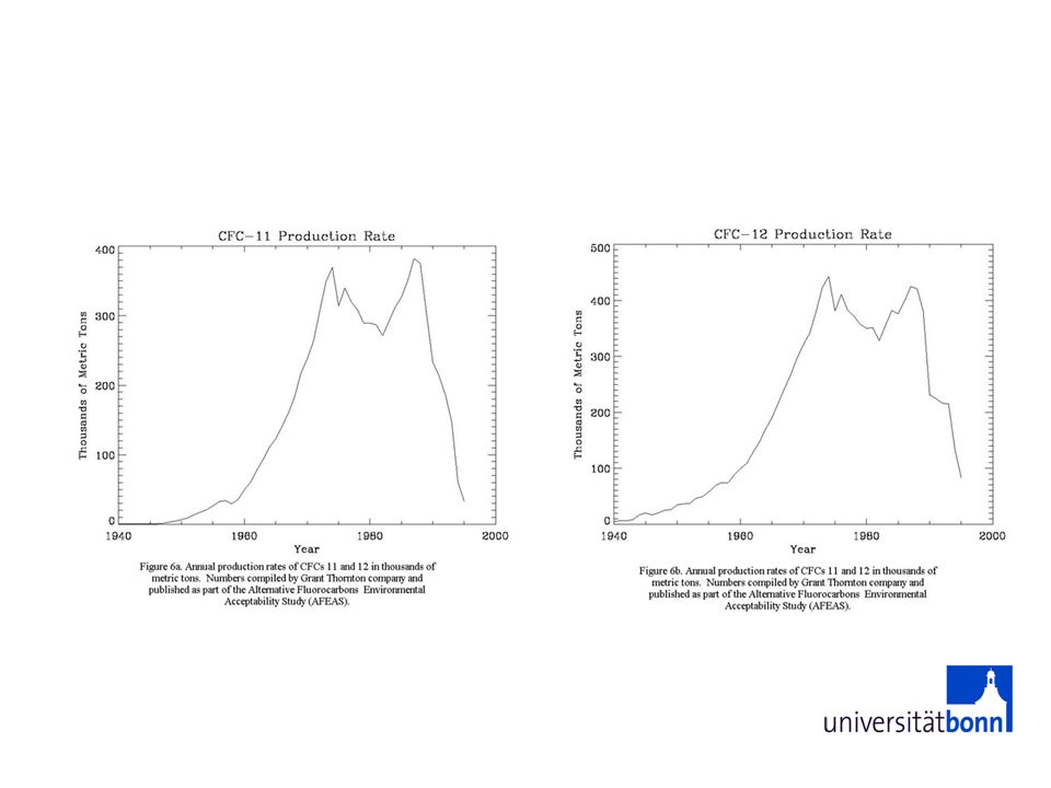
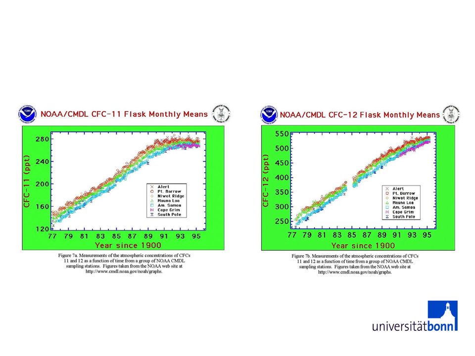
ClOx species (Cl, ClO) are produced from chlorofluorocarbons (CFCs) and methyl chloride (CH3Cl). Example (Freon CF2Cl2): CF2Cl2 + hn CF2Cl + Cl CF2Cl2 + O CF2Cl + ClO Übung: schätze ab OH+CH4 versus O1D+CH4
 are produced from chlorofluorocarbons (CFCs) and methyl chloride (CH3Cl). Example (Freon CF2Cl2): CF2Cl2 + hn CF2Cl + Cl. CF2Cl2 + O CF2Cl + ClO. Übung: schätze ab OH+CH4 versus O1D+CH4.")
32
CFC-01234a (oder HCFC-… oder HFC-…) 0 = Anzahl der Doppelbindungen
Systematik der CFCs CFC-01234a (oder HCFC-… oder HFC-…) 0 = Anzahl der Doppelbindungen (fällt weg, falls keine vorhanden) 1 = Anzahl C-Atome minus 1 (fällt weg, falls Null) 2 = Anzahl H-Atome plus 1 3 = Anzahl F-Atome 4 = Anzahl Cl-Atome, die durch Br ersetzt werden a = Buchstabe zur Identifizierung unterschiedlicher Isomere Die Anzahl Cl-Atome ergibt sich aus der Strukturformel des Ausgangs-Kohlenwasserstoffs.
 0 = Anzahl der Doppelbindungen. (fällt weg, falls keine vorhanden) 1 = Anzahl C-Atome minus 1. (fällt weg, falls Null) 2 = Anzahl H-Atome plus 1. 3 = Anzahl F-Atome. 4 = Anzahl Cl-Atome, die durch Br ersetzt werden. a = Buchstabe zur Identifizierung unterschiedlicher. Isomere. Die Anzahl Cl-Atome ergibt sich aus der Strukturformel. des Ausgangs-Kohlenwasserstoffs.")
33
Beispiele für CFCs CFC-11 CCl3F trichlorofluoromethane
CFC-12 CCl2F2 dichlorodifluoromethane CFC-113 CCl2F-CClF2 1,1,2-trichlorotrifluoroethane HCFC-22 CHClF2 chlorodifluoromethane HCFC-123 CHCl2-CF3 2,2-dichloro-1,1,1-trifluoroethane HCFC-123a CHClF-CClF2 1,2-dichloro-1,1,2-trifluoroethane HFC-23 CHF3 trifluoromethane HFC-134 CHF2-CHF2 1,1,2,2-tetrafluoroethane HFC-134a CH2F-CF3 1,2,2,2-tetrafluoroethane HCFC-20 CHCl3 chloroform Halon-1211 CBrClF2 bromochlorodifluoromethane Quelle: Halone: "CFC" mit Brom-Atomen

35
Reactions of NOx species with O3
ClOx cycle (2) Reactions of NOx species with O3 Cl + O3 ClO + O2 ClO + O Cl + O2 X + O3 XO + O2 XO + O X + O2 net: O + O3 2O2 Nobelpreis Chemie 1995
 Reactions of NOx species with O3. Cl + O3 ClO + O2. ClO + O Cl + O2. X + O3 XO + O2. XO + O X + O2. net: O + O3 2O2. Nobelpreis Chemie")
37
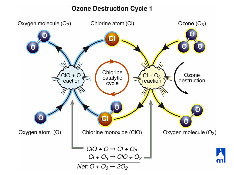
Katalytische Ozonzerstörung
Chapman: O2 + h O + O O + O2 + M O3 + M O3 + h O2 + O O3 + O O2 + O2 Aktivierungsenergie: 17.1 kJ mol-1 Katalytisch (ClOx): Cl + O3 ClO + O2 ClO + O Cl + O2 Aktivierungsenergie: 2.1 kJ mol-1
: Cl + O3 ClO + O2. ClO + O Cl + O2. Aktivierungsenergie: 2.1 kJ mol-1.")
38
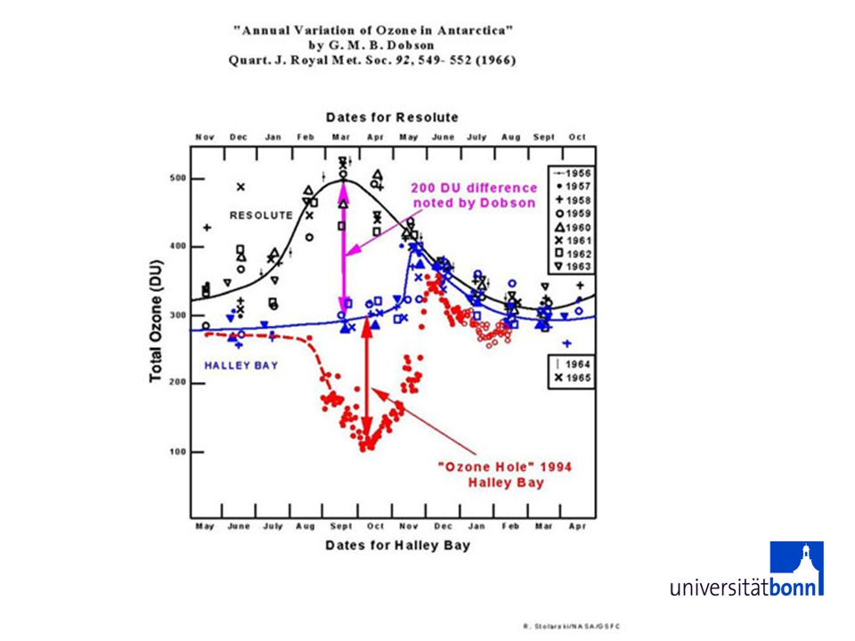
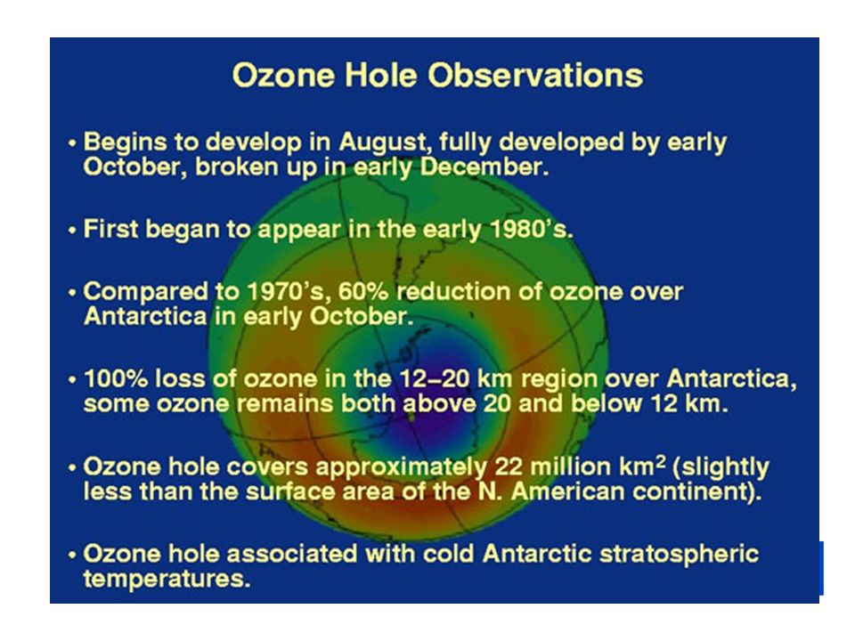
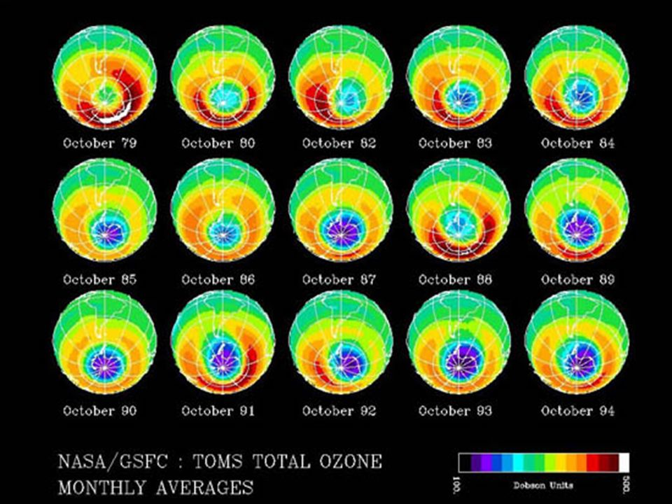
Das Ozonloch

41
Mögliche Übungsaufgabe: Schätze die Gesamtozonsäulendichte aus dem Diagramm ab (mit und ohne Loch)
")
43
WMO Ozone Bulletin

44
Entstehung des Ozonlochs in der Antarktis
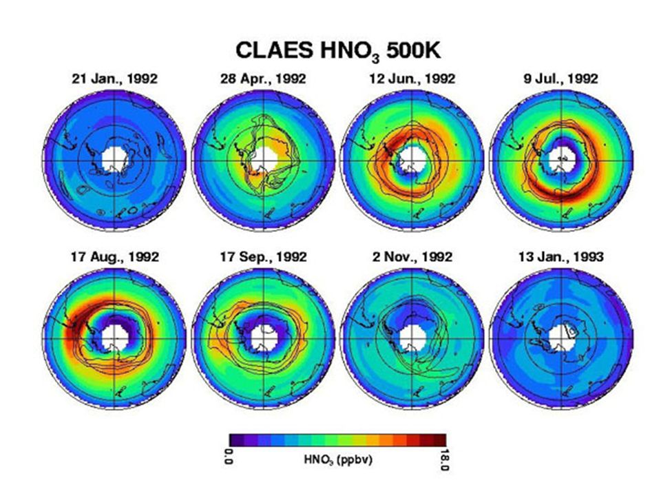
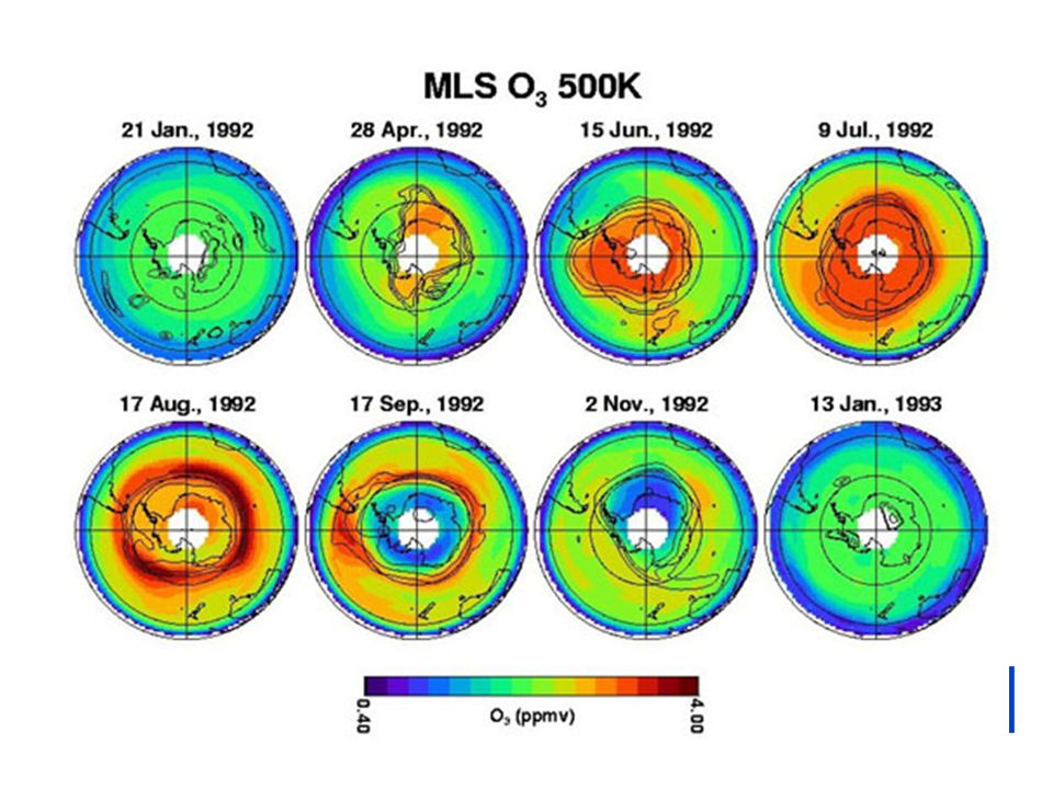
Der zirkumpolare Luftstrom ("polar vortex") im Winter sorgt für eine Isolierung der antarktischen Luftmassen vom Rest der Atmosphäre Extreme Abkühlung durch Abstrahlung (ca. -80C) Bildung von polaren Stratosphärenwolken (PSC) Anlagerung nicht reaktiver Chlorverbindungen (HCl und ClONO2) Heterogene Umwandlung in "aktive" Chlorverbindungen (HOCl und Cl2), die gasförmig freigesetzt werden Mit dem ersten Sonnenlicht im Frühjahr Photolyse der aktiven Chlorverbindungen und katalytische Ozonzerstörung
 im Winter sorgt für eine Isolierung der antarktischen Luftmassen vom Rest der Atmosphäre. Extreme Abkühlung durch Abstrahlung (ca. -80C) Bildung von polaren Stratosphärenwolken (PSC) Anlagerung nicht reaktiver Chlorverbindungen (HCl und ClONO2) Heterogene Umwandlung in aktive Chlorverbindungen (HOCl und Cl2), die gasförmig freigesetzt werden. Mit dem ersten Sonnenlicht im Frühjahr Photolyse der aktiven Chlorverbindungen und katalytische Ozonzerstörung.")
45
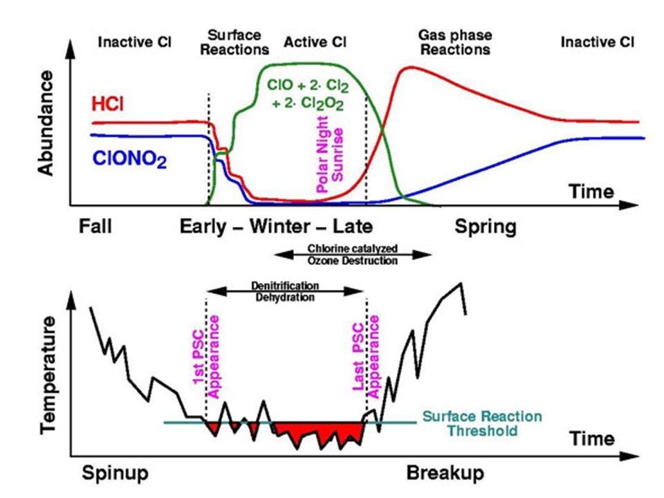
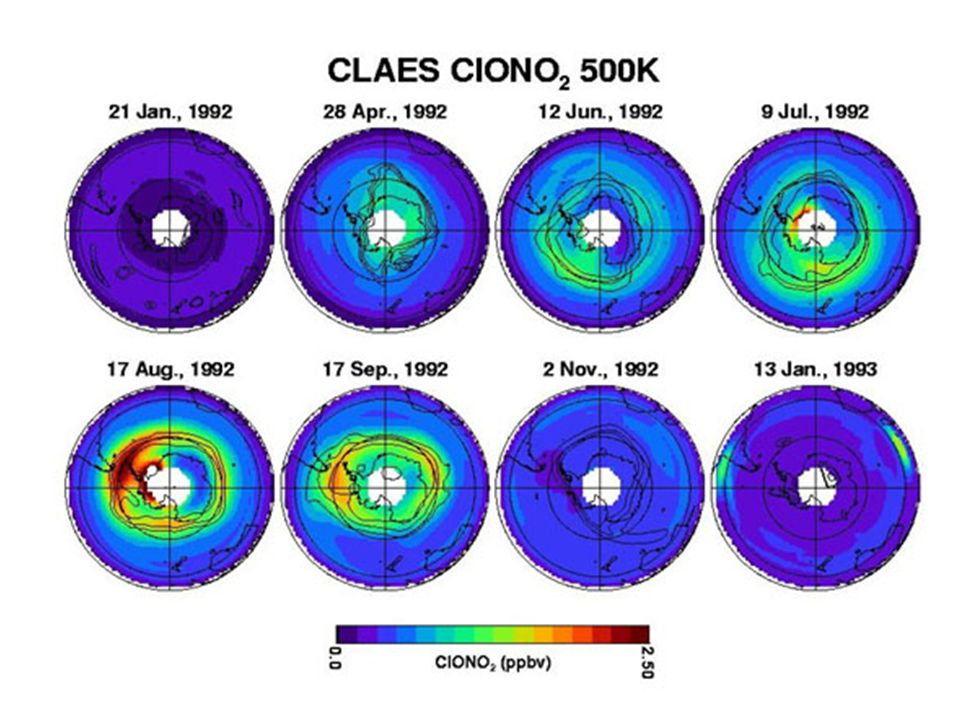
Chlor-Aktivierung

46
Konturlinien: 4K

54
Das Arktische Ozonloch 2011
Zum ersten Mal Ozonzerstörung von ähnlichem Ausmaß wie in der Antarktis Frage: warum bildet sich über der Arktis nicht immer ein Ozonloch?

55
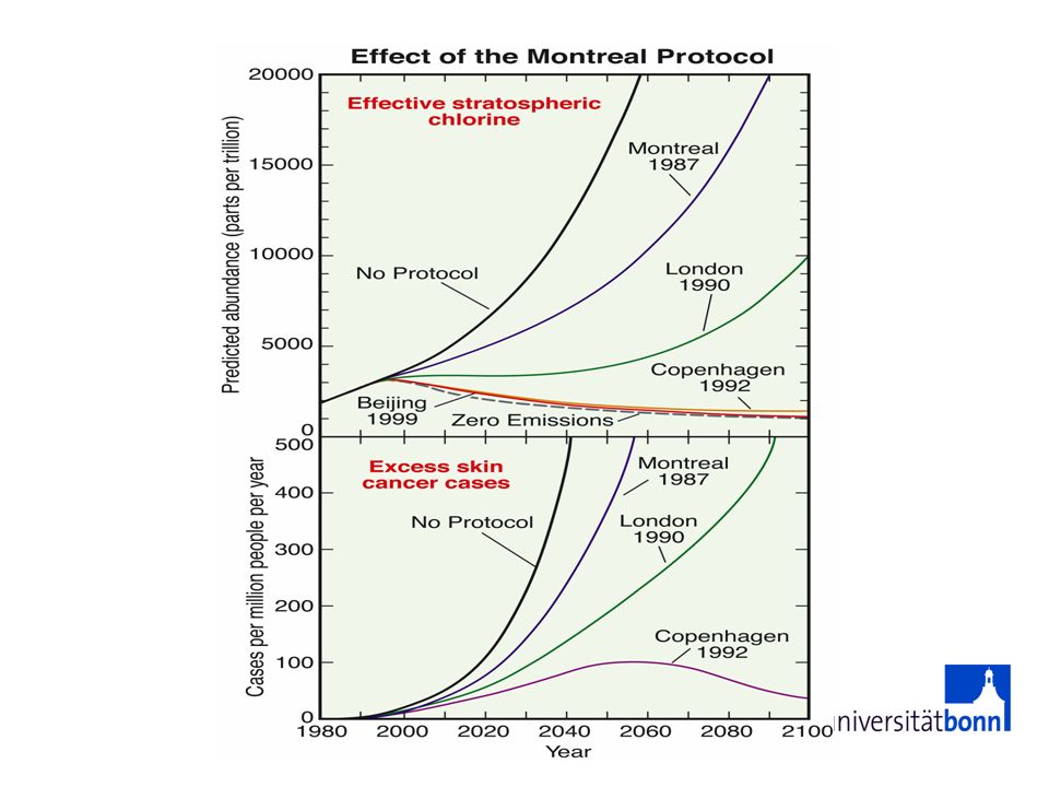
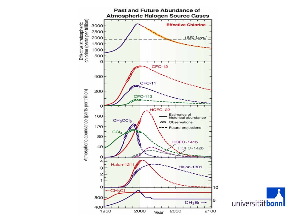
Zukünftige Entwicklung Stratosphärischen Ozons

60
"Super recovery"

61
Modellierung von stratosphärischem Ozon

62
MOZART-3 Model of Ozone and related tracers
Paper by Kinnison et al., 2006 (J. Geophys. Res.) 108 Spezies 218 Gasphasen-Reaktionen 71 Photolyse-Reaktionen 18 Heterogene Reaktionen
 108 Spezies. 218 Gasphasen-Reaktionen. 71 Photolyse-Reaktionen. 18 Heterogene Reaktionen.")
63
MOZART-3 heterogene Reaktionen (1)
(liquid) (solid, T 200 K)
 (solid, T 200 K)")
64
MOZART-3 heterogene Reaktionen (2)
(solid, T 185 K)
")
65
EP TOMS vs MZ3/ECMWF, September 15, 2002
1.25 lon x 1.0 lat 1.9 lon x 1.9 lat For future interactive studies it will be important to derive a reasonable ozone distribution: Daily data from EP TOMS; 1999, blanks where no data 15-day results from WACCM Equatorial region looks very reasonable (260DU- NH winter/spring maximum is derived, DU high. SH winter/spring maximum is off the pole, again WACCM is a little high Ozone hole minimum is in pretty good agreement.

66
EP TOMS vs MZ3/ECMWF, September 25, 2002
1.25 lon x 1.0 lat 1.9 lon x 1.9 lat For future interactive studies it will be important to derive a reasonable ozone distribution: Daily data from EP TOMS; 1999, blanks where no data 15-day results from WACCM Equatorial region looks very reasonable (260DU- NH winter/spring maximum is derived, DU high. SH winter/spring maximum is off the pole, again WACCM is a little high Ozone hole minimum is in pretty good agreement.

Ähnliche Präsentationen


 U N I V E R S I T Ä T H A M B U R G November 2011.>")
Media Landesanstalt für Kommunikation Baden-Württemberg (LFK) Landeszentrale für Medien und Kommunikation.>")


