Vorlesung 12+13: Roter Faden: Wiederholung H-Atom

Präsentation zum Thema: "Vorlesung 12+13: Roter Faden: Wiederholung H-Atom"—  Präsentation transkript:

1 Vorlesung 12+13: Roter Faden: Wiederholung H-Atom
Bahnmagnetismus (Zeeman-Effekt) Spinmagnetismus (Stern-Gerlach-Exp.) Landé-Faktor (Einstein-deHaas Effekt) Spin-Bahn Kopplung (Vektormodell J=L+S) Lamb-Retherford Verschiebung Folien auf dem Web: Siehe auch: Demtröder, Experimentalphysik 3, Springerverlag Und

2 Quantummechanisches Modell des H-Atoms

3 Winkelabhängigkeit der Wellenfkt.

4 Radiale Abhängigkeit der Wellenfkt.

5 Energieniveaus

6 Radiale Bahnen mit l=0

7 Nomenklatur

8 Nomenklatur

9 Nomenklatur

10 Aufhebung der Entartung
Entartung (Kugelsymmetrie) aufgehoben durch: externe B,E-Felder interne B,E-Felder relativ. Korrekturen Vakuumpolarization

11 Ursachen für Abweichung der Kugelsymmetrie
Interne E-Felder: bei mehreren Elektronen schirmen innere Elektronen die Kernladung ab. Kommt später bei Mehrelektron-Atomen. Interne B-Felder: Bewegung der Elektronen erzeugt Strom und damit B-Feld  Bahnmagnetismus. Elektronen haben Eigendrehimpuls (SPIN genannt) (klassisch: Drehbewegung, aber punktförmiges Teilchen hat keine Trägheitsmoment und ist auch nicht quantisiert. Spin ist reiner Quanteneffekt mit Quantenzahlen analog zum Drehimpuls l =½ ħ) Im Labor: 20T erreichbar

12 Experimentelle Befunde: Aufhebung der Entartung
(Zeeman-Effekt)

13 Nobelpreis Zeeman

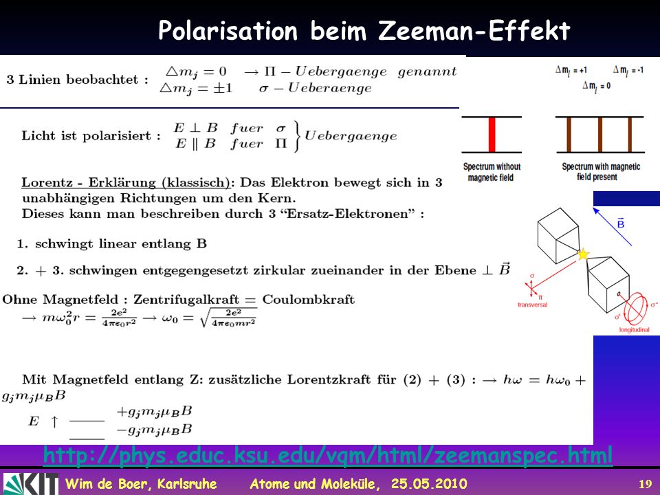
14 Normaler Zeeman-Effekt
Klassisch: drehendes Elektron-> magnetisches Moment p  L QM: Quantisierung von L -> Quantisierung von p -> ‘Kompassnadel’ hat nur bestimmte Einstellungen und Energien!

15 Magnetisches Moment

16 Bahnmagnetismus (klassisches Modell) f f=1/t

17 “Normaler” Zeeman-Effekt (Atome ohne Elektronenspin)
Bahnmagnetismus  Drehimpuls + Quantisierung des Drehimpulses Aufspaltung in diskrete Energieniveaus in äußerem Magnetfeld Zeeman-Effekt ħ

18 “Normaler” Zeeman-Effekt
ħ (J/T=Am2) Anomaler Zeeman-Effekt berücksichtigt Spin (später mehr)

19 Polarisation beim Zeeman-Effekt

20 Zeeman-Effekt

21 Der Elektronenspin (Eigendrehimpuls)

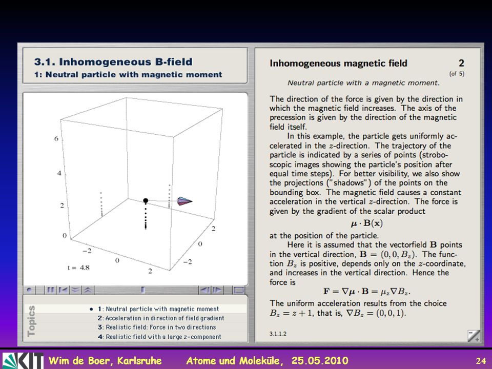
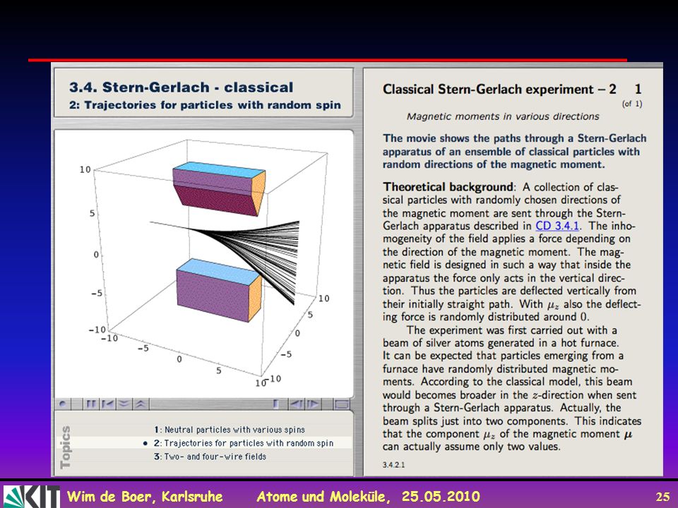
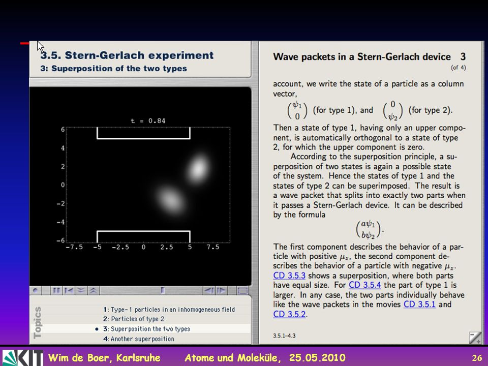
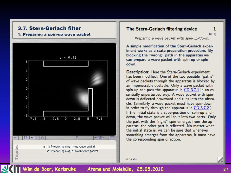
22 Stern-Gerlach Effekt ħ

23 Stern-Gerlach Effekt

24

25

26

27

28 ħ

29 Zusammenfassung aus Stern-Gerlach-Exp. an vielen Atomen

30 Einstein-de Haas-Effekt (Wiki)
The Einstein–de Haas effect is a physical phenomenon delineated by Albert Einstein and Wander Johannes de Haas in the mid 1910's, that exposes a relationship between magnetism, angular momentum, and the spin of elementary particles. The effect corresponds to the mechanical rotation that is induced in a ferromagnetic material (of cylindrical shape and originally at rest), suspended with the aid of a thin string inside a coil, on driving an impulse of electric current through the coil.[1] To this mechanical rotation of the ferromagnetic material (say, iron) is associated a mechanical angular momentum, which, by the law of conservation of angular momentum, must be compensated by an equally large and oppositely directed angular momentum inside the ferromagnetic material. Given the fact that an external magnetic field, here generated by driving electric current through the coil, leads to magnetization of electron spins in the material (or to reversal of electron spins in an already magnetised ferromagnet — provided that the direction of the applied electric current is appropriately chosen), the Einstein–de Haas effect demonstrates that spin angular momentum is indeed of the same nature as the angular momentum of rotating bodies as conceived in classical mechanics. This is remarkable, since electron spin, being quantized, cannot be described within the framework of classical mechanics.

31 Einstein-de Haas-Effekt

32 Magnetisierung

33 Diamagnetismus und Paramagnetismus

34 Einstein-de Haas-Effekt
ħ

35 Einstein-de Haas-Effekt
ħ

36 Zusammenfassung Elektronspin

37 Spin-Bahn-Kopplung VLS

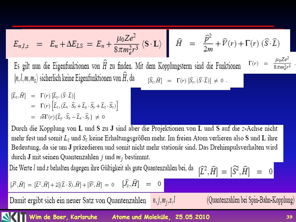
38 Vektormodell der Spin-Bahn-Kopplung

39

40 Vektormodell für J=L+S

41 Zusammenfassung Spin-Bahn-Kopplung

42 Fraunhofer-Linien (Absorptionslinien
in Sonnenlicht, Bunsenbrenner,usw) Die Fraunhoferlinien erlauben Rückschlüsse auf die chemische Zusammensetzung und Tempe-ratur der Gasatmosphäre der Sonne und von Sternen. Gelbe Flamme durch Salz (NaCL) in Flamme

43 Zusammenfassung der Feinstruktur
Problem: bei Wasserstoff Aufspaltung von 2S½ and 2P½ (entdeckt von Lamb und Retherford) Erklärung: Vakuumpol.

44 Relativ. Korrekturen und Lamb-Shift

45 Lamb-Shift durch QED Korrekturen höherer Ordnung

46 Lamb-Shift

47 Lamb-Retherford-Experiment
While the Lamb shift is extremely small and difficult to measure as a splitting in the optical or uv spectral lines, it is possible to make use of transitions directly between the sublevels by going to other regions of the electromagnetic spectrum. Willis Lamb made his measurements of the shift in the microwave region. He formed a beam of hydrogen atoms in the 2s(1/2) state. These atoms could not directly take the transition to the 1s(1/2) state because of the selection rule which requires the orbital angular momentum to change by 1 unit in a transition. Putting the atoms in a magnetic field to split the levels by the Zeeman effect, he exposed the atoms to microwave radiation at 2395 MHz (not too far from the ordinary microwave oven frequency of 2560 MHz). Then he varied the magnetic field until that frequency produced transitions from the 2p(1/2) to 2p(3/2) levels. He could then measure the allowed transition from the 2p(3/2) to the 1s(1/2) state. He used the results to determine that the zero-magnetic field splitting of these levels correspond to 1057 MHz. By the Planck relationship, this told him that the energy separation was E-6 eV.

48 Lamb-Retherford-Experiment

49 Lamb-Retherford-Experiment

50 Lamb-Retherford-Experiment

51 Energieniveaus des H-Atoms mit relativ. Korrekturen
nach Dirac und Feinstruktur der L.S-Kopplung relat. Korr. relat. Korr. + L.S Koppl. Auswahlregel für erlaubte Übergänge: Δl=±1, Δm=0,±1 relat. Korr.

52 n n=3 n=2 Aufhebung der Entartung bei der Wasserstoff Balmer-Linie Hα

53 Zum Mitnehmen Bahnbewegung erzeugt magnetisches Moment pL zum Drehimpuls L Da L quantisiert ist, ist p quantisiert. Dies führt zu diskrete Energieniveaus in einem externen Magnetfeld B mit Splitting mμBB wobei μB das Bohrmagneton ist. Splitting entdeckt von Zeeman. Zusätzlich zu dieses magnetisches Moment durch die Bahnbewegung erzeugt das Elektron auch ein magnetisches Moment durch sein Eigendrehimpus oder Spin S mit pS S. Bahndrehimpuls L und Spin bilden Gesamtdrehimpuls J=L+S, dessen z-Kom-ponente wieder quantisiert ist -> magnetische QZ mj. L und S präzessieren um J und daher tun die „Kompassnadel“ pL und pS dies auch Spin hat g-Faktor = 2,d.h. Eigendrehimpuls ist zweimal so effektiv als Bahndrehimpuls um magnetisches Moment zu erzeugen (klassisch nicht erklärbar, folgt jedoch aus relativ.Wellen-Gleichung (DIRAC-Gleichung)) Energieniveaus nur abhängig von Gesamtdrehimpuls-QZ j, wenn man sehr kleine höhere Ordung Korrekturen (Lamb-Shift) weglässt. Lamb-Shift sehr genau gemesssen-> sehr guter Check für Quantenelektrodynamik QED.