Die Atmosphäre und ihre Veränderungen

Präsentation zum Thema: "Die Atmosphäre und ihre Veränderungen"—  Präsentation transkript:

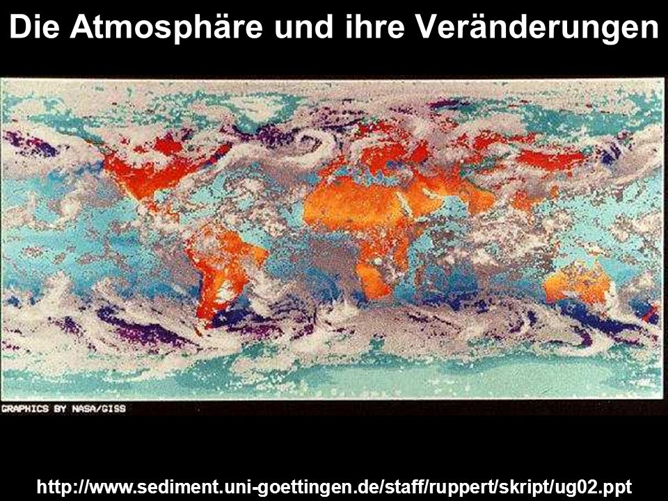
1 Die Atmosphäre und ihre Veränderungen

2 Die Atmosphäre – eine verletzliche Haut

3 http://www. climatescience
Schematic of chemical and transport processes related to atmospheric composition. These processes link the atmosphere with other components of the Earth system, including the oceans, land, and terrestrial and marine plants and animals.

4 Menschen-verursachte (= anthropogene oder technogene) Veränderungen der Atmosphäre und ihre Auswirkungen Ursache Wirkung Emission von Treibhausgasen wie CO2 und CH4 → Treibhauseffekt Emission Ozon-abbauender Substanzen → Ozonloch Emission von Partikeln und Nukleationskeimen → Sichtverminderung, Emission von Säurebildnern (Stickoxide, SO2 etc.)→ Niederschlags-, Boden-, Gewässerversauerung, Waldsterben Emission von Säurebildnern, Partikeln und → photochemischer Smog, reaktiven Gasen Materialkorrosion, Gesund heitsbeeinträchtigung durch Inhalation oder Deposition

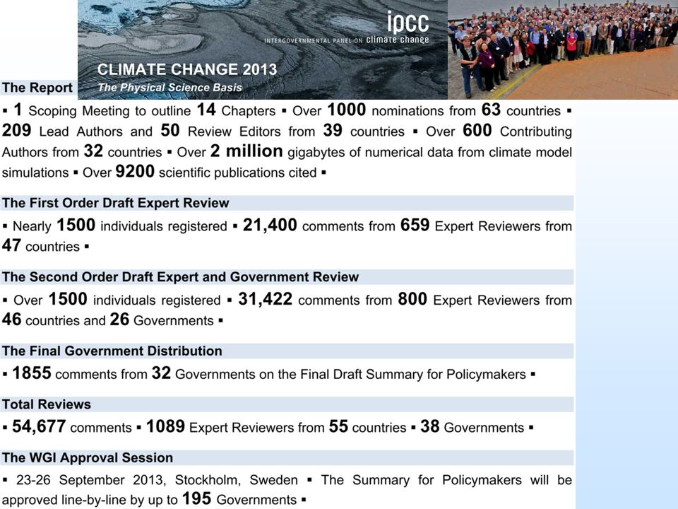
5 http://www.ipcc.ch/report/ar5/wg1/#.UmaovECNAXc (22.10.2013)

6

7 Konzentrationsverlauf der Treibhaus-gase CO2, Methan CH4 und Lachgas N2O in der Erdatmosphäre über die letzten Jahre bis ins Jahr Dabei stammt nur die rote Spitze der Kurve von direkten Messungen in der Atmosphäre. Werte für weiter zurückliegende Zeitpunkte haben Wissenschaftler aus Eisbohrkernen gewonnen. IPCC (2007): natur/0,1518,463865,00.html Radiative forcing is usually quantified as the ‘rate of energy change per unit area of the globe as measured at the top of the atmosphere’, and is expressed in units of ‘Watts per square metre’. When radiative forcing from a factor or group of factors is evaluated as positive, the energy of the Earth-atmosphere system will ultimately increase, leading to a warming of the system.

8 Ice with trapped air bubbles

9 Anthropogenic Perturbation of the Global Carbon Cycle
Perturbation of the global carbon cycle caused by anthropogenic activities, averaged globally for the decade 2002–2011 (PgC/yr) Source: Le Quéré et al. 2012; Global Carbon Project 2012 ( )

10 The current global energy system is dominated by fossil fuels.
On a global basis, it is estimated that renewable Energies accounted for 12.9% of the total 492 Exajoules (EJ) of primary energy supply in 2008. ( )

11 Fate of Anthropogenic CO2 Emissions (2002-2011 average)
8.3±0.4 PgC/yr % 4.3±0.1 PgC/yr 46% 2.6±0.8 PgC/yr 28% Calculated as the residual of all other flux components + 1.0±0.5 PgC/yr % 26% 2.5±0.5 PgC/yr Source: Le Quéré et al. 2012; Global Carbon Project 2012, ( )

12 Global Carbon Budget Emissions to the atmosphere are balanced by the sinks Averaged sinks since 1959: 44% atmosphere, 28% land, 28% ocean ( ) The dashed land-use change line does not include management-climate interactions The land sink was a source in 1987 and 1998 (1997 visible as an emission) Source: Le Quéré et al. 2012; Global Carbon Project 2012

13 Correlation between carbon emissions, CO2 concentrations in the atmosphere and temperature change during the last millenium

14 Mean surface temperature change (°C) from 1901 to 2012
1. The temperature rise increases towards the North. 2. The temperature rise is smaller in the ocean water than on land surfaces. ( ) Annual and five-year running mean temperature change (oC) for both hemispheres relative to the baseline period of The temperature change is more pronounced in the Northern than in the Southern Hemisphere. ( )

15 The warmest 16 years of records:
Global mean temperatures rise faster and faster! The warmest 16 years of records: 1990,1995,1997,2008,2001,2004,2012,2003, 2006,1998,2002,2007,2009,2005,2011,2010 IPCC (2007):

16 Greenhouse gas (CO2,CH4, and N2O) and δ D (deuterium) records for the past yrs. from EPICA Dome C and other ice cores Vostock station Brook (2005): Tiny Bubbles Tell All. Science, 310, 1285 ([D]/[H])sample δD (‰) = 1000 x ([D]/[H]standard The greenhouse gas (CO2,CH4, and N2O) and deuterium (D) records for the past 650,000 years from EPICA Dome C and other ice cores, with marine isotope stage correlations (labeled at lower right) for stages 11 to 16. δD, a proxy for air temperature, is the deuterium/hydrogen ratio of the ice, expressed as a per mil deviation from the value of an isotope standard. More positive values indicate warmer conditions. Data for the past 200 years from other ice core records (20-22) and direct atmospheric measurements at the South Pole are also included. The temperature of the last interglacial Eem (~ BP) could correspond to the temperature at 2100 AD. The sea level was 5-6 m higher than today.

17 Influences of greenhouse gas emissions on climate, land and ocean
2001 2007 2013 2001 2007 2013 Der angegebene Grad der Verlässlichkeit von Schlüsselergebnissen basiert auf der Einschätzung des zugrundeliegenden wissenschaftlichen Verständnisses durch das Autorenteam und wird als Vertrauensniveau ausgedrückt (sehr tief, tief, mittel, hoch und sehr hoch), wenn möglich auch quantitativ mit einer Wahrscheinlichkeitsangabe (praktisch sicher % Wahrscheinlichkeit, äußerst wahrscheinlich %, sehr wahrscheinlich %, wahrscheinlich %, eher wahrscheinlich als nicht %). ( )

18 Reconstructed global-average temperature relative to (blue) and projected global-average temperature out to 2100 (the latter from IPCC, 2007, different scenarios) Mann et al. (2008);

19 total radiative forcing approximate CO2 (CO2-eq.*)
Representative Concentration Pathways (RCPs) For the Fifth Assessment Report of IPCC in Oct. 2013, the scientific community has defined a set of four new scenarios, denoted Representative Concentration Pathways (RCPs). They are identified by their approximate total radiative forcing in year 2100 relative to 1750: total radiative forcing approximate CO2 (CO2-eq.*) 2.6 W m-2 for RCP (475) ppm 4.5 W m-2 for RCP (630) ppm 6.0 W m-2 for RCP (800) ppm 8.5 W m-2 for RCP (1313) ppm *= CO2 including CH4 and N2O ( )

20 Maps representing the model scenarios RCP2. 6 and RCP8
Maps representing the model scenarios RCP2.6 and RCP8.5 in 2081–2100 (a) annual mean surface temperature change, (b) average percent change in annual mean precipitation ( )

21 Potential emissions from remaining fossil resources could result in GHG concentration levels far above 600ppm. ( )

22 Veränderungen durch gesteigerte Temperaturen im 20. Jahrhundert
Zunahme von Niederschlägen in Regionen der mittleren und hohen nördlichen Breiten um 5-10% Zunahme von Extremereignissen wie Starkniederschläge, Hitze- und Dürreperioden, das Abtauen von Gletschern, das Abschmelzen der Masse des Arktischen Eises um 40 %, das Auftauen von Dauerfrostböden (Permafrost), das spätere Zufrieren und frühere Aufbrechen von Flussvereisungen, eine Verschiebung von Lebensräumen bestimmter Tiere und Pflanzen in größere Höhen und polwärts, Übergreifen der Sahara auf S-Spanien, die Dezimierung einiger Tierpopulationen, das frühere Auftreten von Baumblüten, das Auftauchen nicht heimischer (invasiver) Insektenarten und ein verändertes Brut- und Wanderungsverhalten bei Vögeln Zunahme der Bleichung von Korallen Umweltbundesamt (2005): Globaler Klimawandel. S. 7 (ergänzt)

23 Atmosphärenaufbau (mittlere Breiten)
Troposphäre Atmosphärenaufbau (mittlere Breiten) Die Temperatur in der Troposphäre nimmt im Mittel um 6.5 oC pro km ab. Die Troposphäre ist etwa 11 km mächtig (Pole: 9 km, Äquator: bis 18 km). Etwa 3/4 der gesamten Atmosphären-masse befindet sich in der Troposphäre. Nahezu alles Wettergeschehen findet in der Troposphäre statt (dort ist fast alles atmosphärisches H2O). 2001 Brooks/Cole Publishing  temperature

24 Turco (1997, S )

25 Energiebilanz der Erdhülle
( ) Sichtbares Licht gelangt zu etwa einem Drittel direkt an die Erdoberfläche. Ein weiterer Teil wird von der Atmosphäre und den Wolken absorbiert oder reflektiert. Zusätzlich kommt es zu einer Streuung der Strahlung an den Luftmolekülen. Es kommt zu einer diffusen Strahlung aus der Atmosphäre und auch von den Wolken, die – wie bereits erwähnt – Teile der Strahlung absorbiert haben. Letztlich erreicht etwa die Hälfte der Einstrahlung direkt oder indirekt den Erboden. Ein kleiner Teil wird auch hier reflektiert. Der weitaus größte Teil wird jedoch aufgenommen und gespeichert. Es kommt zu einer Erwärmung der Erdoberfläche und damit natürlich auch zu einer langwelligen Wärmestrahlung. Diese wird jedoch nicht direkt wieder an den Weltraum abgegeben sondern von der Atmosphäre als Gegenstrahlung reflektiert. Nur kleine Mengen werden sofort nach außen abgegeben und langfristig strahlt natürlich die Atmosphäre Energie in Form von Wärm ab. Am Ende wird in der Bilanz genau so viel Energie ausgestrahlt, wie auch zugeführt wurde. Innerhalb der Atmosphäre finden ebenfalls noch Energietransporte durch das Wettergeschehen ab, das allerdings seinerseits auch nur durch die Sonnenstrahlung angetrieben wird. Das folgende Schema zeigt das etwa 0,1 Prozent der Einstrahlung in die Fotosynthese der Pflanzen eingeht und damit auch in alle anderen Lebewesen übertragen wird. Die Sonne ist somit der Energielieferant der das Leben für alle Lebewesen erst ermöglicht. Wenn Leben vergeht bleibt immer noch ein Teil der Sonnenenergie in dem organischen Material gespeichert. Diese Sonnenenergie setzen wir bei der Nutzung von fossilen Energieträgern wieder frei.

26 Hansen (2005): Spektrum der Wissenschaft 2/2005, S. 37

27 Global mean energy budget (W/m2) under present day climate conditions.
( ) In summary, newly available observations from both space-borne and surface-based platforms allow a better quantification of the Global Energy Budget, even though notable uncertainties remain, particularly in the estimation of the non-radiative surface energy balance components. Numbers state magnitudes of the individual energy fluxes in W/m2, adjusted within their uncertainty ranges to close the energy budgets. Numbers in parentheses attached to the energy fluxes cover the range of values in line with observational constraints.

28 Globale Windzirkulations-systeme im Schnitt
Idealisiertes 3-Zellen-Zirkulationsmodell

29 Ungefähre Abschätzung charakteristischer Zeiten für den lateralen und vertikalen Austausch zwischen Luft- bzw. Wassermassen Rodhe (1994) in Butcher et al., p. 71 ← WEEKS to 1 MONTH →

30 Selected pollutants, their average residence times in the atmosphere and maximum extent of their impact Maximum scale of the problem ↑ Residence time in the atmosphere → UNEP (2007): Geo-4 Report. Global Environment Outlook GEO4. S. 43. Quelle: EEA 1995, Centre for Airborne Organics 1997

31 The composition of tropospheric air: volume fractions in per cent and parts per million per volume (ppmv) 2013: ~400 ppmv Turco (1997): Earth under Siege. S. 13

32 CH4 (Methan) ca. 0,016 m N2O (Lachgas) ca. 0,0022 m
ca. 2,72m (2008), natürlich 1,97m CH4 (Methan) ca ,016 m N2O (Lachgas) ca ,0022 m Roedel (2000): Physik unserer Umwelt – Die Atmosphäre. S

33 Turco (1997): Earth under Siege. S. 52

34 Sorptionsbereiche typischer Treibhausgase für Strahlung
Mittlere globale Temperatursteigerung durch Treibhausgase von –18 oC auf +15 oC Ausstrahlfenster zwischen ~7-12 µm

35 Turco (1997, S. 338)

36 Bär, M., Blaser, B. et al. (1995): Folienserie des Fonds der Chemischen Industrie. Textheft 22: Umweltbereich Luft. Frankfurt

37 Albedo: [lateinisch albus »weiß«] in Astronomie und Meteorologie ein Maß für das Rückstrahlvermögen von diffus reflektierenden Oberflächen (z.B. der Sonnenstrahlung durch Erdoberfläche und Atmosphäre). (other estimate: 5-10%) Die Albedo der Wolken hängt von verschiedenen Faktoren ab. Hierzu gehören ihre Höhe, ihre Größe und die Anzahl und Größe der in ihnen enthaltenen Tropfen. Die Farbe der Wolken reicht von hellem Weiß zu dunklem Grau, da die Wassertropfen Licht streuen. Große Tropfen haben eine große Oberfläche und reflektieren mehr Licht, als es zahlreiche kleinere Tropfen tun würden. Stehen wir unter einer großen Cumulonimbus-Wolke mit dicken Tropfen, so ist die Umgebung dunkel, da das Licht kaum durch die Wolke kommt. Vom Weltraum aber würde dieselbe Wolke sehr hellweiß aussehen, da sie in Wahrheit eine hohe Albedo hat. Im Gegensatz hierzu ist eine Cirrus-Wolke fast transparent. Vom Weltall aus aber sähe sie grauer aus, da ihre Albedo gering ist. Hohe dünne Wolken wie die Cirrus-Wolken tragen zur Erwärmung bei. Tiefe dicke Wolken wie Stratocumulus hingegen begünstigen eher die Abkühlung. Derzeit nehmen Wissenschaftler an, dass der weltweite Einfluss von Wolken insgesamt die Temperatur der Erde senkt. Wissen darüber zu gewinnen, ob die Wolken im Falle einer globalen Erwärmung durch menschliche Aktivität mehr zur weiteren Erwärmung oder mehr zur gegensteuernden Abkühlung beitragen, ist eine der größten Herausforderungen für die Klimaforschung der Zukunft. Steigt die Temperatur im weltweiten Mittel, so gelangt mehr Wasserdampf in die Luft, demzufolge entstehen auch mehr Wolken. Werden sie mehr Sonnenlicht zurück in den Weltraum streuen oder werden sie mehr Wärmeenergie in der Atmosphäre zurückhalten?

38 Linking relative humidity to cloud feedbacks
(A) Water vapor (in cm), (B) cloud fraction, and (C) reflected solar radiation (in W/m2) for July 2012. Clouds cool the climate by reflecting incoming sunlight back to space, but they also warm the climate by absorbing upwelling terrestrial radiation from the surface. Their net effect is to cool the planet, but changes in clouds in response to global warming may increase or reduce this cooling. Climate models do not agree on the spatial patterns of cloud changes or their net radiative effects, and the cloud feedback is responsible for most of the uncertainty in climate sensitivity in model studies. Observational data are needed to resolve these issues. Black regions in the water vapor plot indicate missing data, often due to high cloud coverage. Regions with high cloud fraction and reflected solar radiation generally coincide with high amounts of water vapor. Note in particular the subtropical regions with low reflected solar radiation. Fasullo & Trenbert (2012) use the correlations of these three fields to relate relative humidity changes to reflected solar radiation changes and, hence, cloud feedbacks. Despite decades of improvements in computer models of Earth's climate, estimates of the climate sensitivity—the change in global average surface air temperature in response to a doubling of carbon dioxide concentration—remain uncertain (1). Much of the uncertainty results from radiative feedbacks that amplify or dampen climate changes. Particular attention has been given to the cloud feedback. Global warming is expected to change the cloud cover, but these changes and their effects on global temperature are very difficult to predict. John T. Fasullo*, Kevin E. Trenberth (2012): A Less Cloudy Future: The Role of Subtropical Subsidence in Climate Sensitivity. Science 9 November 2012: Vol no pp An observable constraint on climate sensitivity, based on variations in mid-tropospheric relative humidity (RH) and their impact on clouds, is proposed. We show that the tropics and subtropics are linked by teleconnections that induce seasonal RH variations that relate strongly to albedo (via clouds), and that this covariability is mimicked in a warming climate. A present-day analogue for future trends is thus identified whereby the intensity of subtropical dry zones in models associated with the boreal monsoon is strongly linked to projected cloud trends, reflected solar radiation, and model sensitivity. Many models, particularly those with low climate sensitivity, fail to adequately resolve these teleconnections and hence are identifiably biased. Improving model fidelity in matching observed variations provides a viable path forward for better predicting future climate. Science 9 November 2012: vol no

39 Does temperature increased water evaporation enhance an atmospheric warming (yellow) or cooling (blue) More vapour or more clouds? This schematic illustrates just two out of the dozens of climate feedbacks identified by scientists. The warming created by greenhouse gases leads to additional evaporation of water into the atmosphere. But water vapour itself is a greenhouse gas and can cause even more warming (steps 2-4 are repeated). Scientists call this “positive water-vapor feedback.” On the other hand, if the water vapor leads to the formation of more clouds, some warming may be counteracted because clouds reflect solar radiation (steps 5-8). Clouds also trap heat in the atmosphere. A major research question is how many and what type of clouds will form—low clouds tend to cool (reflect more energy than they trap) and high clouds tend to warm (trap more energy than they reflect).

40 ↑ Annual cycle of CO2 in the northern hemisphere
 Concentration trends of carbon dioxide CO2 (top) and methane CH4 (bottom) in the atmosphere Decay of org. mat. Photo-synthesis Decay of organic material Jan. April July Oct. Jan. ↑ Annual cycle of CO2 in the northern hemisphere CH4 is emitted by many industrial processes (ruminant farming, rice agriculture, biomass burning, coal mining, and gas & oil industry) and by natural reservoirs (wetlands, permafrost and peatlands). Annual industrial emissions of CH4 are not available as they are difficult to quantify. CH4 emissions from natural reservoirs can increase under warming conditions. This has been observed from permafrost thawing in Sweden. If the CH4 increase is caused by the response of natural reservoirs to warming, it could continue for decades to centuries and enhance the greenhouse gas burden of the atmosphere. CO2 and CH4 are the two most important anthropogenic greenhouse gases. The trends with seasonal cycle removed are shown in red.

41 Pre-industrial and recent (2011) greenhouse gas concentrations in the tropo-sphere
Blasing (2012): Carbon Dioxide Information Analysis Center; ( ) Global warming potential (GWP) expresses a gas’s heat-trapping power relative to carbon dioxide over a particular time period. For CO2 the specification of an atmospheric lifetime is complicated by the numerous removal processes involved, which necessitate complex modeling of the decay curve. Because the decay curve depends on the model used and the assumptions incorporated therein, it is difficult to specify an exact atmospheric lifetime for CO2. Accepted values range around 100 years.

42 Classes of Compounds of Halocarbons
Chlorofluorocarbons (CFCs): when derived from methane and ethane these compounds have the formulae CClmF4-m and C2ClmF6-m, where m is nonzero. Hydrochlorofluorocarbons (HCFCs): when derived from methane and ethane these compounds have the formulae CClmFnH4-m-n and C2ClxFyH6-x-y, where m, n, x, and y are nonzero (commercial: e.g. Freon). Bromochlorofluorocarbons and bromofluorocarbons have formulae similar to the CFCs and HCFCs but also bromine (commercial: e.g. halones). Hydrofluorocarbons (HFCs): when derived from methane, ethane, propane, and butane, these compounds have the respective formulae CFmH4-m, C2FmH6-m, C3FmH8-m, and C4FmH10-m, where m is nonzero. Perfluorinated compounds (PFCs) refer to a class of organofluorine compounds that have all hydrogens replaced with fluorine on a carbon chain.

43 Shares of anthropogenic sources of global greenhouse gas emissions in 2010 (50.1 GtCO2e) by main sector and gas type (in CO2-equivalent) ( ); McKeown & Gradner (2009): Climate Change Reference Guide. Worldwatch Institute, 17 pp. The primary human-generated greenhouse gases are CO2, CH4, fluorinated gases (including CFCs = chlorofluorocarbons), N2O, and O3. Greenhouse gases are only one source of climate change; aerosols such as black carbon, sulfuric acid, and solar radiation also affect warming.

44 Shares of anthropogenic sources of global greenhouse gas emissions in 2010 (50.1 GtCO2e) by main sector (in CO2-equivalent) ( ); McKeown & Gradner (2009): Climate Change Reference Guide. Worldwatch Institute, 17 pp.

45 Trend in global greenhouse gas emissions 1970-2010 by sector
Trend in global greenhouse gas emissions by sector . This graph shows emissions of 50.1 Gt CO2eq in 2010. ( )

46 CO2-Emissionen (1980 und 1989) in Abhängigkeit vom Breitengrad
Agnew et al. (2004): An Introduction to Environmental Chemistry. S. 252

47 Global Carbon Storage in Above- and Below-Ground Live Vegetation
1 ha = m2 World Resources Institute and PAGE (2000) Despite constant exchanges of C between forest biomass, soils, and the atmosphere, a large amount is always present in leaves and woody tissue, roots, and soils. This quanti-ty of C is known as the carbon store. C sequestration and storage slow the rate at which CO2 accumulates in the atmosphere and mitigate global warming billion tons of C are estimated to be stored in the world’s above- and below-ground live vegetation.

48 Global Carbon Storage in Soils
(World Resources Institute and PAGE, 2000) WRI’s estimates of carbon stores in soils are based on those of Batjes (Batjes, 1996), who estimated the global stock of organic carbon in the upper 100 cm of the soil to be between 1,462 and 1,548 billion tons of carbon. Carbon storage values in the boreal region reach a maximum of 1250 metric tons of carbon per hectare.

49 Global carbon storage in above- and below-ground live vegetation and soils (World Resources Institute and PAGE, 2000) The carbon store depicted in this map is 2,385 billion tons. The low-end estimate is 1,752 billion tons (World Resources Institute and PAGE, 2000). Forest ecosystems account for about 40 % of the total carbon, about 34 % is stored in grasslands, about 17 % in agricultural lands. The highest quantities of stored carbon are located in the tropical and boreal forest regions. In the tropics, more carbon is stored in vegetation than in soils while in the boreal region far more carbon is stored in the soils. Peatlands in the boreal region are especially important areas because of the large quantities of soil carbon stored per unit area. (11/2011)

50 Sources of CO2 emissions from global land use change 2000
Baumert et al (2005) Afforestation: establishment of a forest or stand of trees in an area where there was no forest. Reforestation: reestablishment of forests, either naturally or artificially (direct seeding or planting)

51 Temporal evolution of the atmospheric carbon balance over the years Red line: CO2 emissions from fossil fuel burning. ( ) The atmospheric accumulation shows a large interannual variability, which is caused by corresponding strong variations in terrestrial CO2 uptake, while the ocean uptake, globally, does not vary much from year to year. This interannual variability is driven primarily by climate variations. Drought conditions in important large terrestrial ecosystems, e.g. in the Amazonas basin during El Niño phases induce carbon losses by decreased photosynthesis, increased decomposition and/or increased wildfires. These losses show up in the atmosphere as anomalous CO2 increases during these years. The interannual variability is driven primarily by climate variations. Drought conditions in important large terrestrial ecosystems, e.g. in the Amazonas basin during El Niño phases induce carbon losses by decreased photosynthesis, increased decomposition and/or increased wildfires.

52 Increase in global temperatures may both increase and decrease the atmospheric CO2. content:
Scenario 1: Rising temperatures facilitate the release of soil carbon from organic matter, which is oxidized to CO2. Scenario 2: However, increased temperature also leads to increased growth in plants, which absorb CO2 (if enough water is available).

53 Sarmiento & Gruber (2002)

54 ← Annual methane emissions from anthropogenic and natural sources
( ) Annual methane sinks ↓ Total CH4 yearly flux for → ( )

55 The amount of aerosols in the air has direct effect on the amount of solar radiation hitting the Earth's surface. Aerosols may have significant local or regional impact on temperature. Water vapour is a greenhouse gas, but at the same time the upper white surface of clouds reflects solar radiation back into space. Albedo - reflections of solar radiation from surfaces on the Earth - creates difficulties in exact calculations. If e.g. the polar icecap melts, the albedo will be significantly reduced. Open water absorbs heat, while white ice and snow reflect it. IPCC (2001)

56 Sonnenaktivität und Klima
Man muss über Jahre in der Erdgeschich-te zurückgehen, bis man einen Zeitraum findet, in dem die Sonne im Mittel ebenso aktiv war wie in den vergangenen 60 Jahren (Basis 14C). (8.11/2012) Sonnenfleckenhäufigkeit (10 Jahres-Mittelwerte seit der Eiszeit) Sonnenflecken erscheinen dunkel, weil das starke Magnetfeld den Energietrans-port durch Gasströmungen aus dem Son-neninneren unterdrückt (~1500oC kühler). Eine Abnahme der Aktivität wird in wenigen Jahrzehnten erwartet. Es ist offen, inwieweit diese Aktivitäten das Klima beeinflussen. vergrößerter Ausschnitt Die Menge des produzierten C-14 hängt stark von der Zahl der Teilchen der kosmischen Strahlung ab, welche die Erdatmosphäre erreichen. Diese Zahl wiederum schwankt mit der Stärke der Sonnenaktivität: Ist die Aktivität höher, so bildet das Magnetfeld der Sonne einen effektiven Schutzschild gegen diese Teilchen, ist die Aktivität geringer, steigt die Intensität der kosmischen Strahlung an. Folglich wird bei höherer Sonnenaktivität weniger und bei geringerer Sonnenaktivität mehr C-14 produziert. Die primäre kosmische Strahlung ist aufgrund ihrer kosmischen Entstehung von besonderem astronomischen Interesse. Sie besteht aus hochenergetischen Partikeln, besonders Protonen (85%) und Alphateilchen (14%) sowie schweren Atomkernen. Ein kleiner Anteil der kosmischen Strahlung wird von der Sonne erzeugt (Energie etwa eV). Die kosmische Strahlung mittlerer Energie ( eV) stammt aus dem Milchstraßensystem (z.B. von Supernovae und deren Überresten, den Pulsaren, sowie aus dem Kern der Milchstraße), während die energiereichste kosmische Strahlung (bis 1020 eV) v.a. aus den aktiven Kernen anderer Galaxien stammt. Sami K. Solanki, Ilya G. Usoskin, Bernd Kromer, Manfred Schüssler, Jürg Beer: Unusual activity of the Sun during recent decades compared to the previous 11,000 years. Nature, 28 October 2004

57 Bestimmt die wechselnde Sonnenaktivität unser Klima
Bestimmt die wechselnde Sonnenaktivität unser Klima? Verlauf der mittleren Temperatur der Atmosphäre und der Strahlungsleistung der Sonne: Zwischen beiden Größen gibt es nur bis etwa 1980 auffallende Parallelen. Max-Planck-Institut für Sonnensystemforschung (2005) (8.11/2012) Oben rechts: Die Sonne im Licht einer ultravioletten Emissionslinie des neutralen Heliums, die bei Kelvin ausgestrahlt wird. In dem dunkleren Gebiet um die Polkappe - dem koronalen Loch - liegen die Quellen des schnellen Sonnenwindes, der von der Sonne aus in die Heliosphäre bläst. Unten: Die Gesamthelligkeit der Sonne folgt einem 11-jährigen Zyklus schwankt um 0.1 % (bedingt durch wechselndes Magnetfeld). Gewaltige Eruptionen auf der Sonne schleudern Wolken aus Gas und Magnetfeldern in den Weltraum und auch auf das irdische Magnetfeld. Besonders starke Sonnenstürme können diesen natürlichen Schutzschild durchbrechen und so zu intensiven Polarlichtern, aber auch zur Beeinträchtigung des Funkverkehrs und möglichen Beschädigungen von Kommunikationssatelliten, Telefon- und Hochspannungsleitungen führen.

58 main drivers of climate change.
Radiative forcing estimates in relative to and aggregated uncertaini-ties for the main drivers of climate change. ( )