Die Atmosphäre und ihre Veränderungen

Präsentation zum Thema: "Die Atmosphäre und ihre Veränderungen"—  Präsentation transkript:

1 Die Atmosphäre und ihre Veränderungen http://www.sediment.uni-goettingen.de/staff/ruppert/skript/ug02.ppt

2

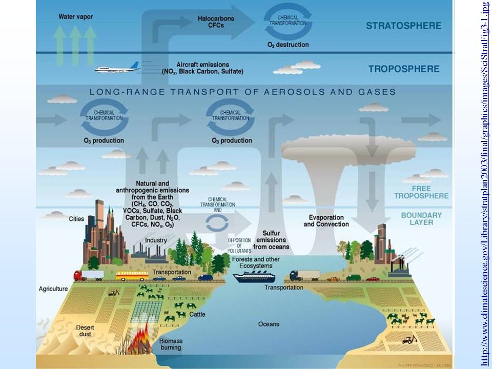
3 http://www.climatescience.gov/Library/stratplan2003/final/graphics/images/SciStratFig3-1.jpg

4 Menschen-verursachte (= anthropogene oder technogene) Veränderungen der Atmosphäre und ihre Auswirkungen Emission von Treibhausgasen wie CO 2 und CH 4 → Treibhauseffekt Emission Ozon-abbauender Substanzen→ Ozonloch Emission von Partikeln und Nukleationskeimen → Sichtverminderung, Emission von Säurebildnern (Stickoxide, SO 2 etc.)→ Niederschlags-, Boden-, Gewässerversauerung, Waldsterben Emission von Säurebildnern, Partikeln und → photochemischer Smog, reaktiven Gasen Materialkorrosion, Gesund- heitsbeeinträchtigung durch Inhalation oder Deposition Ursache Wirkung

5 http://www.ipcc.ch/report/ar5/wg1/#.UmaovECNAXchttp://www.ipcc.ch/report/ar5/wg1/#.UmaovECNAXc (22.10.2013)

6 http://ipcc.ch/pdf/presentations/ar5/wg1/plattner13geneva_gen.pdfhttp://ipcc.ch/pdf/presentations/ar5/wg1/plattner13geneva_gen.pdf (7.11.2013)

7 IPCC (2007): http://www.spiegel.de/wissenschaft/ natur/0,1518,463865,00.htmlttp://www.spiegel.de/wissenschaft/ natur/0,1518,463865,00.html Konzentrationsverlauf der Treib- hausgase CO 2, Methan CH 4 und Lachgas N 2 O in der Erdatmosphäre über die letzten 10000 Jahre bis 2005. Dabei stammt nur die rote Spitze der Kurve von direkten Messungen in der Atmosphäre. Werte für weiter zurück- liegende Zeitpunkte wurden aus Eisbohrkernen gewonnen.

8 Greenhouse gas (CO 2,CH 4, and N 2 O) and δ D (deuterium) records for the past 650000 yrs. from EPICA Dome C and other ice cores Brook (2005): Tiny Bubbles Tell All. Science, 310, 1285 The temperature of the last interglacial Eem (~120 000 BP) could correspond to the temperature at 2100 AD. The sea level was 5-6 m higher than today. Vostock station ([D]/[H]) sample δD (‰) = 1000 x ------------------ -1 ([D]/[H] standard

9 Ice with trapped air bubbles

10  Ice cores Tree rings  Tools for reconstructing the climate of the past Glacier retreats and advances In paleoclimatology climate proxies deliver approximations that suggest the climate patterns of the past before direct measurements. Examples: ice cores - tree rings – corals – deposits of mires, lake, caves, and ocean - glacier lengths, historical sources. Systematic cross-verification between proxies is necessary. National Academies Report (2008): "Understanding and Responding to Climate Change” http://www.nationalacademies.org/morenews/20080519.htmlhttp://www.nationalacademies.org/morenews/20080519.html (March 2010)

11 http://www.wmo.int/pages/prog/arep/gaw/ghg/documents/GHG_Bulletin_10_Nov2014_EN.pdflhttp://www.wmo.int/pages/prog/arep/gaw/ghg/documents/GHG_Bulletin_10_Nov2014_EN.pdfl (4.11.2015)

12 Anthropogenic Perturbation of the Global Carbon Cycle averaged globally for the decade 2004–2013 (GtCO 2 /yr) Source: CDIAC; NOAA-ESRL; Le Quéré et al 2014; Global Carbon Budget 2014 http://www.globalcarbonproject.org/carbonbudget/14/files/GCP_budget_2014_v1.02.pptxhttp://www.globalcarbonproject.org/carbonbudget/14/files/GCP_budget_2014_v1.02.pptx (11.11.2014)

13 Fate of Anthropogenic CO 2 Emissions (2004-2013 average) CDIACCDIAC; NOAA-ESRL; Houghton et al 2012; Giglio et al 2013; Le Quéré et al 2014; Global Carbon Budget 2014NOAA-ESRLHoughton et al 2012Giglio et al 2013Le Quéré et al 2014Global Carbon Budget 2014 http://www.globalcarbonproject.org/carbonbudget/14/files/GCP_budget_2014_v1.02.pptxhttp://www.globalcarbonproject.org/carbonbudget/14/files/GCP_budget_2014_v1.02.pptx (Dec. 17 2014) 9.4±1.8 GtCO 2 /yr 26% 32.4±1.6 GtCO 2 /yr 91% 3.3±1.8 GtCO 2 /yr 9% 10.6±2.9 GtCO 2 /yr 29% Calculated as the residual of all other flux components 15.8±0.4 GtCO 2 /yr 44%

14 Global Carbon Budget Emissions are partitioned between the atmosphere, land, and ocean Source: CDIAC; NOAA-ESRL; Houghton et al 2012; Giglio et al 2013; Joos et al 2013; Khatiwala et al 2013; Le Quéré et al 2014; Global Carbon Budget 2014CDIACNOAA-ESRLHoughton et al 2012Giglio et al 2013Joos et al 2013Khatiwala et al 2013 Le Quéré et al 2014Global Carbon Budget 2014 http://www.globalcarbonproject.org/carbonbudget/14/files/GCP_budget_2014_v1.02.pptxhttp://www.globalcarbonproject.org/carbonbudget/14/files/GCP_budget_2014_v1.02.pptx (Dec. 17 2014)

15 Global Carbon Budget The cumulative contributions to the Global Carbon Budget from 1870 Contributions are shown in parts per million (ppm) Figure concept from Shrink That Footprint Source: CDIAC; NOAA-ESRL; Houghton et al 2012; Giglio et al 2013; Joos et al 2013; Khatiwala et al 2013; Le Quéré et al 2014; Global Carbon Budget 2014 http://www.globalcarbonproject.org/carbonbudget/14/files/GCP_budget_2014_v1.02.pptxhttp://www.globalcarbonproject.org/carbonbudget/14/files/GCP_budget_2014_v1.02.pptx (11.11.2015)

16 Fossil Fuel and Cement Emissions Global fossil fuel and cement emissions: 36.1 ± 1.8 GtCO 2 in 2013, 61% over 1990 Projection for 2014 : 37.0 ± 1.9 GtCO 2, 65% over 1990 Uncertainty is ±5% for one standard deviation (IPCC “likely” range); Estimates for 2011 - 2014 are preliminary. Source: CDIAC; NOAA-ESRL; Le Quéré et al 2014; Global Carbon Budget 2014CDIACNOAA-ESRLLe Quéré et al 2014Global Carbon Budget 2014 http://www.globalcarbonproject.org/carbonbudget/14/files/GCP_budget_2014_v1.02.pptxhttp://www.globalcarbonproject.org/carbonbudget/14/files/GCP_budget_2014_v1.02.pptx (Dec. 17 2014)

17 Modern global anthropogenic carbon emissions from burning fossil fuels Oben: Mak Thope: http://en.wikipedia.org/wiki/Greenhouse_gas (8.3.2015)http://en.wikipedia.org/wiki/Greenhouse_gas Rechts: http://www.ipcc.ch/pdf/assessment-report/ar5/syr/SYR_AR5_SPMcorr2.pdf (8.3.2015)http://www.ipcc.ch/pdf/assessment-report/ar5/syr/SYR_AR5_SPMcorr2.pdf

18 The current global energy system is dominated by fossil fuels. http://srren.ipcc-wg3.de/ipcc-srren-generic-presentation-1http://srren.ipcc-wg3.de/ipcc-srren-generic-presentation-1 (20.9.2012) On a global basis, it is estimated that renewable Energies accounted for 12.9% of the total 492 Exajoules (EJ) of primary energy supply in 2008.

19 Potential emissions from remaining fossil resources could result in GHG concentration levels far above 600ppm. http://srren.ipcc-wg3.de/ipcc-srren-generic-presentation-1http://srren.ipcc-wg3.de/ipcc-srren-generic-presentation-1 (20.9.2012)

20 Top Fossil Fuel Emitters (Absolute) The top four emitters in 2013 covered 58% of global emissions China (28%), United States (14%), EU28 (10%), India (7%) Source: CDIAC; Le Quéré et al 2014; Global Carbon Budget 2014CDIACLe Quéré et al 2014Global Carbon Budget 2014 http://www.globalcarbonproject.org/carbonbudget/14/files/GCP_budget_2014_v1.02.pptxhttp://www.globalcarbonproject.org/carbonbudget/14/files/GCP_budget_2014_v1.02.pptx (Dec. 17 2014)

21 Top Fossil Fuel Emitters (Per Capita) China’s per capita emissions have passed the EU28 and are 45% above the global average Source: CDIAC; Le Quéré et al 2014; Global Carbon Budget 2014CDIACLe Quéré et al 2014Global Carbon Budget 2014 http://www.globalcarbonproject.org/carbonbudget/14/files/GCP_budget_2014_v1.02.pptxhttp://www.globalcarbonproject.org/carbonbudget/14/files/GCP_budget_2014_v1.02.pptx (Dec. 17 2014) Per capita emissions in 2013

22 Correlation between carbon emissions, CO 2 concentrations in the atmosphere and temperature change during the last millenium 2014: 400 ppm

23 Global Annual Mean Surface Air Temperature Change (Land-Ocean) base period: 1951-1980. The green bars show uncertainty estimates. 2014: 14,6 o C The warmest 15 years of records: 2008, 2001, 2004, 2011, 2003, 2002, 2006, 2012, 1998, 2009, 2007, 2013, 2005, 2010, 2014 http://data.giss.nasa.gov/gistemp/graphs_v3/http://data.giss.nasa.gov/gistemp/graphs_v3/ (25.10.2015)

24 http://data.giss.nasa.gov/gistemp/graphs_v3/http://data.giss.nasa.gov/gistemp/graphs_v3/ (11.11.2015) Global Annual Mean Surface Air Temperature Change (Land-Ocean) for the northern and southern hemisphere base period: 1951-1980

25 Die Temperatur in der Troposphäre nimmt im Mittel um 6.5 o C pro km ab. Die Troposphäre ist etwa 11 km mächtig (Pole: 9 km, Äquator: bis 18 km). Etwa 3/4 der gesamten Atmosphären- masse befindet sich in der Troposphäre. Nahezu alles Wettergeschehen findet in der Troposphäre statt (dort ist fast alles atmosphärisches H 2 O). Troposphäre Atmosphärenaufbau (mittlere Breiten)  temperature 2001 Brooks/Cole Publishing

26 Turco (1997): Earth under Siege. S. 13 2013: ~400 ppmv The composition of tropospheric air: volume fractions in per cent and parts per million per volume (ppmv)

27 ca. 2,72m (2008), natürlich 1,97m Roedel (2000): Physik unserer Umwelt – Die Atmosphäre. S. 13-14 CH 4 (Methan) ca. 0,016 m N 2 O (Lachgas) ca. 0,0022 m

28 Turco (1997, S. 326+328)

29 Turco (1997): Earth under Siege. S. 52

30 Ausstrahlfenster zwischen ~7-12 µm Sorptionsbereiche typischer Treibhausgase für Strahlung Mittlere globale Temperatursteigerung durch Treibhausgase von –18 o C auf +15 o C

31 Turco (1997, S. 338)

32 Bär, M., Blaser, B. et al. (1995): Folienserie des Fonds der Chemischen Industrie. Textheft 22: Umweltbereich Luft. Frankfurt

33 http://www.fakko.de/school/sonne/erde_c.htmhttp://www.fakko.de/school/sonne/erde_c.htm (8.11.2012) Energiebilanz der Erdhülle

34 Hansen (2005): Spektrum der Wissenschaft 2/2005, S. 37 IPCC (2013): Der Strahlungsantrieb aller Treibhausgase liegt zwischen 1,1 und 3,3 W m -2 (Durchschnitt 2,3), der Antrieb nur von CO 2 zwischen 1,3 und 2,0 W m -2 (1,7).

35 Global mean energy budget (W/m 2 ) under present day climate conditions. Numbers state magnitudes of the individual energy fluxes in W/m 2, adjusted within their uncertainty ranges to close the energy budgets. Numbers in parentheses attached to the energy fluxes cover the range of values in line with observational constraints. http://data.giss.nasa.gov/gistemp/graphs_v3/http://data.giss.nasa.gov/gistemp/graphs_v3/ (22.10.2013)

36 Pre-industrial and recent (2013) greenhouse gas concentrations in the troposphere Blasing (2014): Recent Greenhouse Gas Concentrations. http://cdiac.ornl.gov/pns/current_ghg.html (4.11.2015) http://cdiac.ornl.gov/pns/current_ghg.html

37 Classes of Compounds of Halocarbons Chlorofluorocarbons (CFCs): when derived from methane and ethane these compounds have the formulae CCl m F 4-m and C 2 Cl m F 6-m, where m is nonzero. Hydrochlorofluorocarbons (HCFCs): when derived from methane and ethane these compounds have the formulae CCl m F n H 4-m-n and C 2 Cl x F y H 6-x-y, where m, n, x, and y are nonzero (commercial: e.g. Freon). Bromochlorofluorocarbons and bromofluorocarbons have formulae similar to the CFCs and HCFCs but also bromine (commercial: e.g. halones). Hydrofluorocarbons (HFCs): when derived from methane, ethane, propane, and butane, these compounds have the respective formulae CF m H 4-m, C 2 F m H 6-m, C 3 F m H 8-m, and C 4 F m H 10-m, where m is nonzero. Perfluorinated compounds (PFCs) refer to a class of organofluorine compounds that have all hydrogens replaced with fluorine on a carbon chain.

38 Residence time in the atmosphere → Maximum scale of the problem Quelle: EEA 1995, Centre for Airborne Organics 1997 Selected pollutants, their average residence times in the atmosphere and maximum extent of their impact UNEP (2007): Geo-4 Report. Global Environment Outlook GEO 4. S. 43. ↑

39 Globale Windzirkulations- systeme im Schnitt Idealisiertes 3-Zellen-Zirkulationsmodell http://www.earth.rochester.edu/fehnlab/ees215/fig15_1.jpg

40 Rodhe (1994) in Butcher et al., p. 71 Ungefähre Abschätzung charakteristischer Zeiten für den lateralen und vertikalen Austausch zwischen Luft- bzw. Wassermassen ← WEEKS to 1 MONTH →

41 Schätzwerte für den Strahlungs- antriebs im Jahr 2011 bezogen auf 1750 sowie kumulative Unsicherheit en für die Haupttreiber des Klima- wandels. https://www.ipcc.ch/pdf/reports-nonUN-translations/deutch/ar5-wg1-spm.pdfhttps://www.ipcc.ch/pdf/reports-nonUN-translations/deutch/ar5-wg1-spm.pdf (9.3.2015) Vertrauens- niveau des Nettoantriebs: SH = sehr hoch, H = hoch, M = mittel, T = gering, ST = sehr gering

42 For the Fifth Assessment Report of IPCC in Oct. 2013, the scientific community has defined a set of four new scenarios, denoted Representative Concentration Pathways (RCPs). They are identified by their approximate total radiative forcing in year 2100 relative to 1750: total radiative forcing approximate CO 2 (CO 2 -eq.*) 2.6 W m -2 for RCP2.6 421 (475) ppm 4.5 W m -2 for RCP4.5538 (630) ppm 6.0 W m -2 for RCP6.0670 (800) ppm 8.5 W m -2 for RCP8.5 936 (1313) ppm *= CO 2 including CH 4 and N 2 O http://www.ipcc.ch/report/ar5/wg1/#.UmaovECNAXchttp://www.ipcc.ch/report/ar5/wg1/#.UmaovECNAXc (22.10.2013) Representative Concentration Pathways (RCPs)

43  Observed changes in global annual average surface temperatures based on trends between 1901-2012. Projected changes in global annual average surface temperature at the end of the 21th century relative to the 1986-2005 mean http://www.de- ipcc.de/_media/WG2AR5_SPM_FI NAL.pdfhttp://www.de- ipcc.de/_media/WG2AR5_SPM_FI NAL.pdf (9.3.2015)

44 http://www.ipcc.ch/report/ar5/wg1/#.UmaovECNAXchttp://www.ipcc.ch/report/ar5/wg1/#.UmaovECNAXc (22.10.2013) Maps representing the model scenarios RCP2.6 and RCP8.5 in 2081–2100 (a) annual mean surface temperature change, (b) average percent change in annual mean precipitation

45 Influences of greenhouse gas emissions on climate, land and ocean http://www.ipcc.ch/report/ar5/wg1/#.UmaovECNAXchttp://www.ipcc.ch/report/ar5/wg1/#.UmaovECNAXc (22.10.2013) 2007 2013 2001 2007 2013 2001

46 “Pillow diagram” used in the US National Assessment to denote fuzzy boundaries to the categories of certainty and uncertainty used (National Assessment Synthesis Team, 2001).

47 http://www.de-ipcc.de/_media/WG2AR5_SPM_FINAL.pdfhttp://www.de-ipcc.de/_media/WG2AR5_SPM_FINAL.pdf (9.3.2015) Risks for Europe from climate change and the potential for reducing risks through adaptation and mitigation. Each key risk is characterized as very low to very high for three timeframes: the present, near term (2030–2040), and longer term (2080–2100). For the longer term, risk levels are presented for a 2°C and 4°C global mean temperature increase above preindustrial levels.

48 http://jamaica.u.arizona.edu/ic/nats1011/lectures/ch03/FIG03_006.JPG Albedo: [lateinisch albus »weiß«] in Astronomie und Meteorologie ein Maß für das Rückstrahlvermögen von diffus reflektierenden Oberflächen (z.B. der Sonnenstrahlung durch Erdoberfläche und Atmosphäre). http://www.atmosphere.mpg.de/enid/3__Sonne_und_Wolken/-_Albedo_3ao.html (other estimate: 5-10%)

49 Linking relative humidity to cloud feedbacks (A) Water vapor (in cm), (B) cloud fraction, and (C) reflected solar radiation (in W/m 2 ) for July 2012. Clouds cool the climate by reflecting incoming sunlight back to space, but they also warm the climate by absorbing upwelling terrestrial radiation from the surface. Their net effect is to cool the planet, but changes in clouds in response to global warming may increase or reduce this cooling. Climate models do not agree on the spatial patterns of cloud changes or their net radiative effects, and the cloud feedback is responsible for most of the uncertainty in climate sensitivity in model studies. Observational data are needed to resolve these issues. Black regions in the water vapor plot indicate missing data, often due to high cloud coverage. Regions with high cloud fraction and reflected solar radiation generally coincide with high amounts of water vapor. Note in particular the subtropical regions with low reflected solar radiation. Fasullo & Trenbert (2012) use the correlations of these three fields to relate relative humidity changes to reflected solar radiation changes and, hence, cloud feedbacks. Science 9 November 2012: vol. 338 no. 6108 755-756

50 Does temperature increased water evaporation enhance an atmospheric warming (yellow) or cooling (blue) http://dels.nas.edu/dels/rpt_briefs/climate-change-final.pdf

51  Concentration trends of carbon dioxide CO 2 (top) and methane CH 4 (bottom) in the atmosphere http://www.copenhagendiagnosis.org ↑ Annual cycle of CO 2 in the northern hemisphere CO 2 and CH 4 are the two most important anthropogenic greenhouse gases. The trends with seasonal cycle removed are shown in red. Jan. April July Oct. Jan. Photo- synthesis Decay of org. mat. Decay of organic material

52 Shares of anthropogenic sources of global greenhouse gas emissions in 2010 (50.1 GtCO 2 e) by main sector and gas type (in CO 2 -equivalent) http://www.unep.org/pdf/2012gapreport.pdfhttp://www.unep.org/pdf/2012gapreport.pdf (22.11.2012); McKeown & Gradner (2009): Climate Change Reference Guide. Worldwatch Institute, 17 pp. The primary human-generated greenhouse gases are CO 2, CH 4, fluorinated gases (including CFCs = chlorofluorocarbons), N 2 O, and O 3. Greenhouse gases are only one source of climate change; aerosols such as black carbon, sulfuric acid, and solar radiation also affect warming.

53 http://www.unep.org/pdf/2012gapreport.pdfhttp://www.unep.org/pdf/2012gapreport.pdf (22.11.2012); McKeown & Gradner (2009): Climate Change Reference Guide. Worldwatch Institute, 17 pp. Shares of anthropogenic sources of global greenhouse gas emissions in 2010 (50.1 GtCO 2 e) by main sector (in CO 2 -equivalent)

54 Trend in global greenhouse gas emissions 1970-2010 by sector. This graph shows emissions of 50.1 Gt CO 2 eq in 2010. http://www.unep.org/pdf/2012gapreport.pdfhttp://www.unep.org/pdf/2012gapreport.pdf (22.11.2012)

55 Agnew et al. (2004): An Introduction to Environmental Chemistry. S. 252 CO 2 -Emissionen (1980 und 1989) in Abhängigkeit vom Breitengrad

56 Global Carbon Storage in Above- and Below-Ground Live Vegetation Despite constant exchanges of C between forest biomass, soils, and the atmosphere, a large amount is always present in leaves and woody tissue, roots, and soils. This quanti- ty of C is known as the carbon store. C sequestration and storage slow the rate at which CO 2 accumulates in the atmosphere and mitigate global warming. 268-901 billion tons of C are estimated to be stored in the world’s above- and below-ground live vegetation. 1 ha = 10 000 m 2 http://earthtrends.wri.org/maps_spatial/maps_detail_static.php?map_select=225&theme=3 World Resources Institute and PAGE (2000)

57 Global Carbon Storage in Soils (World Resources Institute and PAGE, 2000) http://earthtrends.wri.org/maps_spatial/maps_detail_static.cfm?map_select=226&theme=3 WRI’s estimates of carbon stores in soils are based on those of Batjes (Batjes, 1996), who estimated the global stock of organic carbon in the upper 100 cm of the soil to be between 1,462 and 1,548 billion tons of carbon. Carbon storage values in the boreal region reach a maximum of 1250 metric tons of carbon per hectare.

58 http://earthtrends.wri.org/maps_spatial/maps_detail_static.cfm?map_select=227&theme=3http://earthtrends.wri.org/maps_spatial/maps_detail_static.cfm?map_select=227&theme=3 (11/2011) The carbon store depicted in this map is 2,385 billion tons. The low-end estimate is 1,752 billion tons (World Resources Institute and PAGE, 2000). Forest ecosystems account for about 40 % of the total carbon, about 34 % is stored in grasslands, about 17 % in agricultural lands. The highest quantities of stored carbon are located in the tropical and boreal forest regions. In the tropics, more carbon is stored in vegetation than in soils while in the boreal region far more carbon is stored in the soils. Peatlands in the boreal region are especially important areas because of the large quantities of soil carbon stored per unit area. Global carbon storage in above- and below-ground live vegetation and soils (World Resources Institute and PAGE, 2000)

59 Global average atmospheric CO 2 growth rate Atmospheric growth rate of CO 2 as a function of latitude http://www.ipcc.ch/pdf/assessment- report/ar5/wg1/WG1AR5_ALL_FIN AL.pdfhttp://www.ipcc.ch/pdf/assessment- report/ar5/wg1/WG1AR5_ALL_FIN AL.pdf (9.5.2015)

60 Increase in global temperatures may both increase and decrease the atmospheric CO 2. content: Scenario 1: Rising temperatures facilitate the release of soil carbon from organic matter, which is oxidized to CO 2. http:// earthobservatory.nasa.gov/Study/Conundrum / Scenario 2: However, increased temperature also leads to increased growth in plants, which absorb CO 2 (if enough water is available).

61 Sarmiento & Gruber (2002)

62 Maps of storage rate distribution of anthropogenic carbon (mol m –2 y –1 ) for the three ocean basins averaged over 1980–2005. Note that a different color scale is used in each basin. http://www.ipcc.ch/report/ar5/wg1/#.UmaovECNAXchttp://www.ipcc.ch/report/ar5/wg1/#.UmaovECNAXc (22.10.2013)

63 ← Annual methane emissions from anthropogenic and natural sources Annual methane sinks ↓ http://www.carboscope.eu/?q=methane_budget http://www.carboscope.eu/?q=methane_budget (1.11.2013) Total CH 4 yearly flux for 2000- 2005 → http://www.carboscope.eu/?q=flux_map&param=ch4http://www.carboscope.eu/?q=flux_map&param=ch4 (1.11.2013)

64 Schematic of the global cycle of CH 4. Numbers represent annual fluxes in Tg(CH 4 ) yr –1 estima- ted for the time period 2000–2009 and CH 4 reservoirs in Tg(CH 4 ) (1Tg = 10 12 g). Black arrows denote ‘natural’ fluxes, i.e., fluxes that are not directly caused by human activities since 1750, red arrows anthropogenic fluxes, and the light brown arrow denotes a combined natural+anthropogenic flux. Average atmospheric increase each year between 2000–2009: 2.2 ppb yr -1

65 Estimated annual average emissions for the major global methane sources over the period 2000–2009 from Kirschke et al. (2013) The estimate for each source is calculated as the mean of a variable number of individual studies for each source. The range (in brackets) is defined as the maximum and minimum values from the studies reviewed by Kirschke et al. (2013). http://www.amap.no/documents/downloa d/2487http://www.amap.no/documents/downloa d/2487 (11.11.2015)

66 Globally averaged growth rate of atmospheric CH 4 in ppb yr –1 Atmospheric growth rate of CH 4 as a function of latitude http://www.ipcc.ch/report/ar5/wg1 /#.UmaovECNAXchttp://www.ipcc.ch/report/ar5/wg1 /#.UmaovECNAXc (22.10.2013)

67 Schlesinger ( 2013): Biogeochemistry. Elsevier.

68 Intensive Landwirtschaft verschlechtert Klimabilanz Unter Berücksichtigung der CH 4 - und N 2 O- Emissionen aus der Viehhaltung und intensiven Landwirtschaft bei der THG-Bilanz setzen Wälder, Gras- und Ackerland vor allem in Mitteleuropa Treibhausgase frei (in CO 2 -Äquivalenten). Sie nivellieren fast völlig den Effekt, den etwa russische Wälder als CO 2 -Speicher ausüben. E. D. Schulze, S. Luyssaert, P. Ciais, A. Freibauer, I. A. Janssens et al. (2009): Importance of methane and nitrous oxide for Europe's terrestrial greenhouse-gas balance. Nature Geoscience, 22.11 2009; http://idw-online.de/pages/de/news345521http://idw-online.de/pages/de/news345521

69 Figures are averages for the period 2001-2010 www.fao.org/assets/infographics/FAO-Infographic-GHG-en.pdfwww.fao.org/assets/infographics/FAO-Infographic-GHG-en.pdf (4.11.2015) CH 4 CH 4 + N 2 O CH 4 N2ON2O N2ON2O CH 4 + N 2 O FAO (2014): Agriculture, Forestry and Other Land Use Emissions by Sources and Removals by Sinks. 89pp http://www.fao.org/docrep/019/i3671e/i3671e.pdf (5.11.2015) Agricultural activities release a lot of GHG

70 Historical trends in GHG emission intensity, by agricultural commodities, 1961-2010 FAO (2014): Agriculture, Forestry and Other Land Use Emissions by Sources and Removals by Sinks. 89pp http://www.fao.org/docrep/019/i3671e/i3671e.pdf (5.11.2015)

71 (a) Total food intake by region and (b) regional and global per capita food intake carbon  Global total food intake in 2011 was estimated to be 0.57 ± 0.03 Pg C yr -1. The difference between food intake and food supply quantities reported by FAOSTAT indicates that an additional 0.26 Pg C yr -1 or 31% of total food supply is lost from the food supply chain.  Global average per capita food intake carbon has increased over the 51 years of available data. Wolf et al. (2015): Biogenic carbon fluxes from global agricultural production and consumption. Global Biogeochemical Cycles 29, 1617–1639, doi:10.1002/2015GB005119.

72 Globally averaged dry-air mole fractions at Earth’s surface of the major halogen-containing well-mixed GHG HFC-23 (CHF 3 ), HFC-134a (CF 3 CH 2 F), HFC-152a (CH 3 CHF 2 ) ….. http://www.ipcc.ch/report/ar5/wg1/#.UmaovECNA Xchttp://www.ipcc.ch/report/ar5/wg1/#.UmaovECNA Xc (22.10.2013)

73 IPCC (2001)

74 Aerosole - kleinste in der Luft schwebende Partikel – beeinflussen den globalen Strahlungshaushalt direkt durch Absorption und Streuung, sowie indirekt durch Änderung der Wolkeneigenschaften. http://www.dkrz.de/dkrz/gallery/vis/atmosphere.htmlhttp://www.dkrz.de/dkrz/gallery/vis/atmosphere.html (2006) Entwicklung, Interaktion und Ausbreitung verschiedener Aerosole aus unterschied- lichen Quellen über ein Jahr

75 Sonnenflecken erscheinen dunkel, weil das starke Magnetfeld den Energietrans- port durch Gasströmungen aus dem Son- neninneren unterdrückt (~1500 o C kühler). Man muss über 8.000 Jahre in der Erdgeschich- te zurückgehen, bis man einen Zeitraum findet, in dem die Sonne im Mittel ebenso aktiv war wie in den vergangenen 60 Jahren (Basis 14 C). Sonnenaktivität und Klima Sami K. Solanki, Ilya G. Usoskin, Bernd Kromer, Manfred Schüssler, Jürg Beer: Unusual activity of the Sun during recent decades compared to the previous 11,000 years. Nature, 28 October 2004 Eine Abnahme der Aktivität wird in wenigen Jahrzehnten erwartet. Es ist offen, inwieweit diese Aktivitäten das Klima beeinflussen. Sonnenfleckenhäufigkeit (10 Jahres- Mittelwerte seit der Eiszeit) vergrößerter Ausschnitt http://www.mps.mpg.de/de/forschung/sonne/ http://www.mps.mpg.de/de/forschung/sonne/ (8.11/2012)

76 Bestimmt die wechselnde Sonnenaktivität unser Klima? Verlauf der mittleren Temperatur der Atmosphäre und der Strahlungsleistung der Sonne: Zwischen beiden Größen gibt es nur bis etwa 1980 auffallende Parallelen. http://www.mps.mpg.de/de/forschung/sonne/http://www.mps.mpg.de/de/forschung/sonne/ (8.11/2012)Max-Planck-Institut für Sonnensystemforschung (2005)

77 Schätzwerte für den Strahlungs- antriebs im Jahr 2011 bezogen auf 1750 sowie kumulative Unsicherheit en für die Haupttreiber des Klima- wandels. https://www.ipcc.ch/pdf/reports-nonUN-translations/deutch/ar5-wg1-spm.pdfhttps://www.ipcc.ch/pdf/reports-nonUN-translations/deutch/ar5-wg1-spm.pdf (9.3.2015) Vertrauens- niveau des Nettoantriebs: SH = sehr hoch, H = hoch, M = mittel, T = gering, ST = sehr gering